1  What is Time Series Analysis?

1.1 What is time series data?

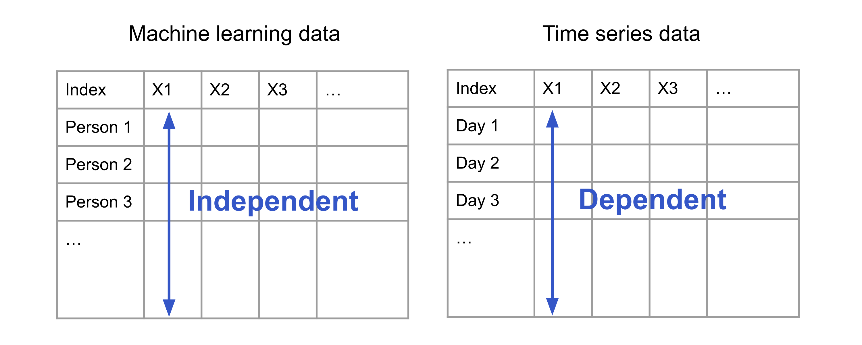
In supervised learning or supervised learning, we work with datasets in which each row is a measurement of a different unit. These could be images of handwritten digits, physical measurements of different plants belonging to the same species, or information about people collected via census. Here, it is reasonable to assume that the rows are independent and identically distributed (i.i.d.) draws from a population. Indeed, the success of the familiar machine learning pipeline, including sample splitting, model fitting, hyperparameter optimization, and model evaluation, hinges on the validity of this assumption.

Unfortunately, as we will see in the examples below, many datasets of interest do not follow this format. Instead, their rows may comprise measurements of the same unit (person, company, country, etc.), made at different points in time. This measurement structure introduces dependencies between the rows, thereby violating the critical i.i.d. assumption (see Figure 1.1.) Over the last century, statisticians, mathematicians, economists, engineers, computer scientists, and researchers in other fields have studied how to overcome the difficulties of working with dependent data points and to exploit the opportunities offered by such structure.

Time series analysis is the name of the subfield studying such data under the further assumption that the measurements are made at regularly-spaced intervals. With time as the row index, each column in such a dataset is called a time series. A dataset comprising possibly multiple time series is called time series data.

Figure 1.1: Time series data contain dependencies across rows.

1.2 Examples of time series

Time series data is truly ubiquitous and appears across disparate domains. To give the reader a sense of this ubiquity, we will list a few examples in this section.

1.2.1 Finance

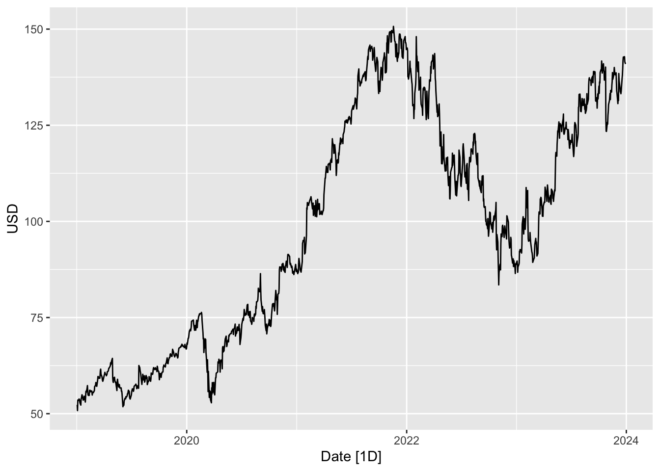
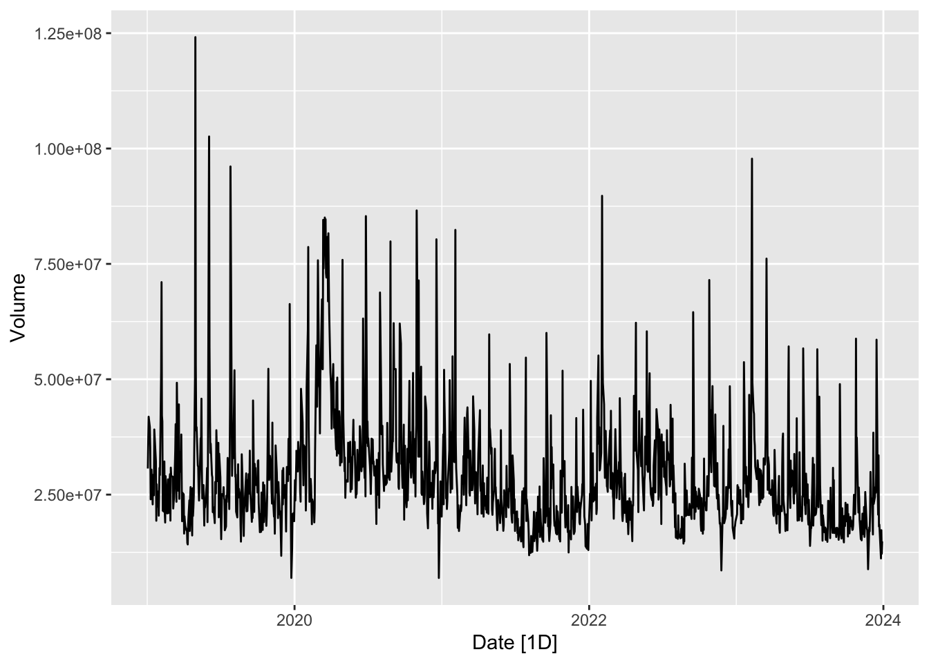
In finance, various types of time series data are commonly analyzed to gain insights into market behavior, assess risk, and make informed investment decisions. Examples include the prices of stocks and derivatives, trading volumes, and exchange rates. The two plots in this section show the price and trading volume of Google’s stock, measured daily, over a five year period from 2 Jan 2019 to 1 Jan 2024. ¹

Figure 1.2: Daily closing value for Google stock.

Figure 1.3: Daily trading volume for Google stock.

1.2.2 Economics and other social sciences

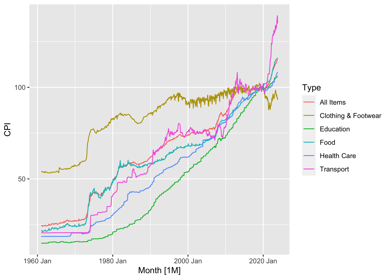
To diagnose the health of the economy and to guide policymakers in making appropriate economic policies, economists keep track of economic indicators such as the Gross Domestic Product (GDP), Consumer Price Index (CPI), unemployment rates, foreign direct investment, and interest rates. The following figure plots the consumer price index for several categories of goods in Singapore, measured quarterly, between 1960 and 2020. 2019 is used as the base year. ²

Figure 1.4: Consumer price index (CPI) in Singapore for several categories of goods, measured quarterly, between 1960 and 2020.

Time series data is also important and prevalent in other social sciences, for instance population dynamics, education outcomes, political opinion polls, crime rates, and cultural trends.

1.2.3 Business

Businesses increasingly collect various streams of data either deliberately or as a by-product of their daily operations. These can then be used to make informed business decisions and to improve busines efficiency, such as through better inventory management. Examples of data streams include sales data, website traffic, user engagement, and quality control metrics.

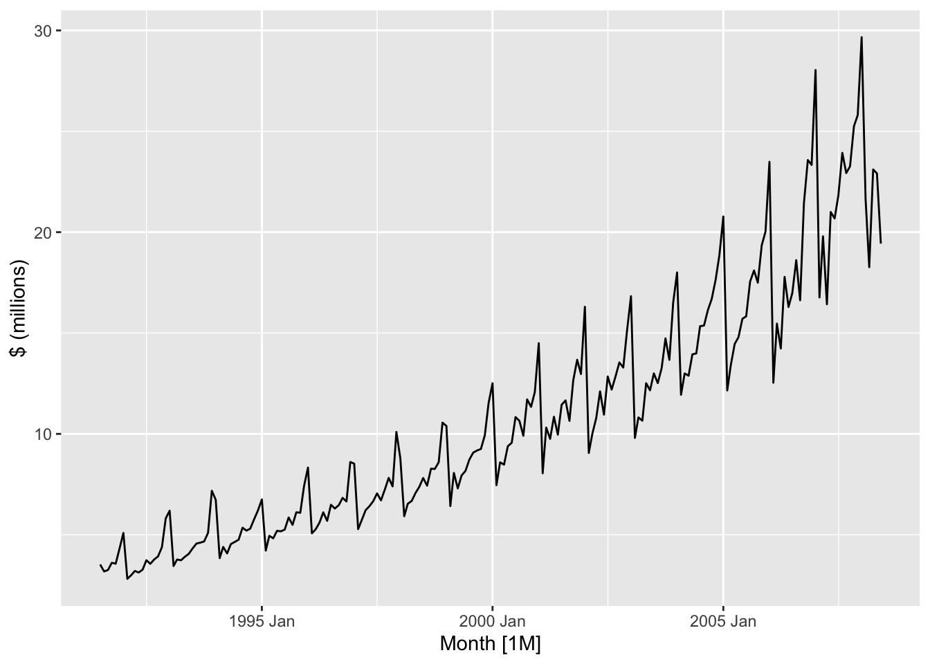
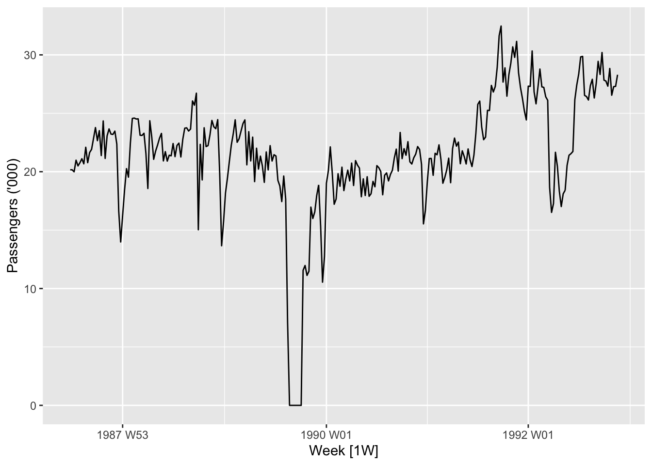
Two such time series are plotted in the next two figures. In Figure 1.5, we plot the sales numbers for antidabetic drugs in Australia, per month, between 1991 and 2008. In Figure 1.6, we plot the weekly number of economy class passengers on Ansett airlines between Melbourne and Sydney between 1987 and 1992. ³

Figure 1.5: Sales numbers for antidabetic drugs in Australia.

Figure 1.6: Weekly number of economy class passengers on Ansett airlines between Melbourne and Sydney.

1.2.4 Environmental sciences

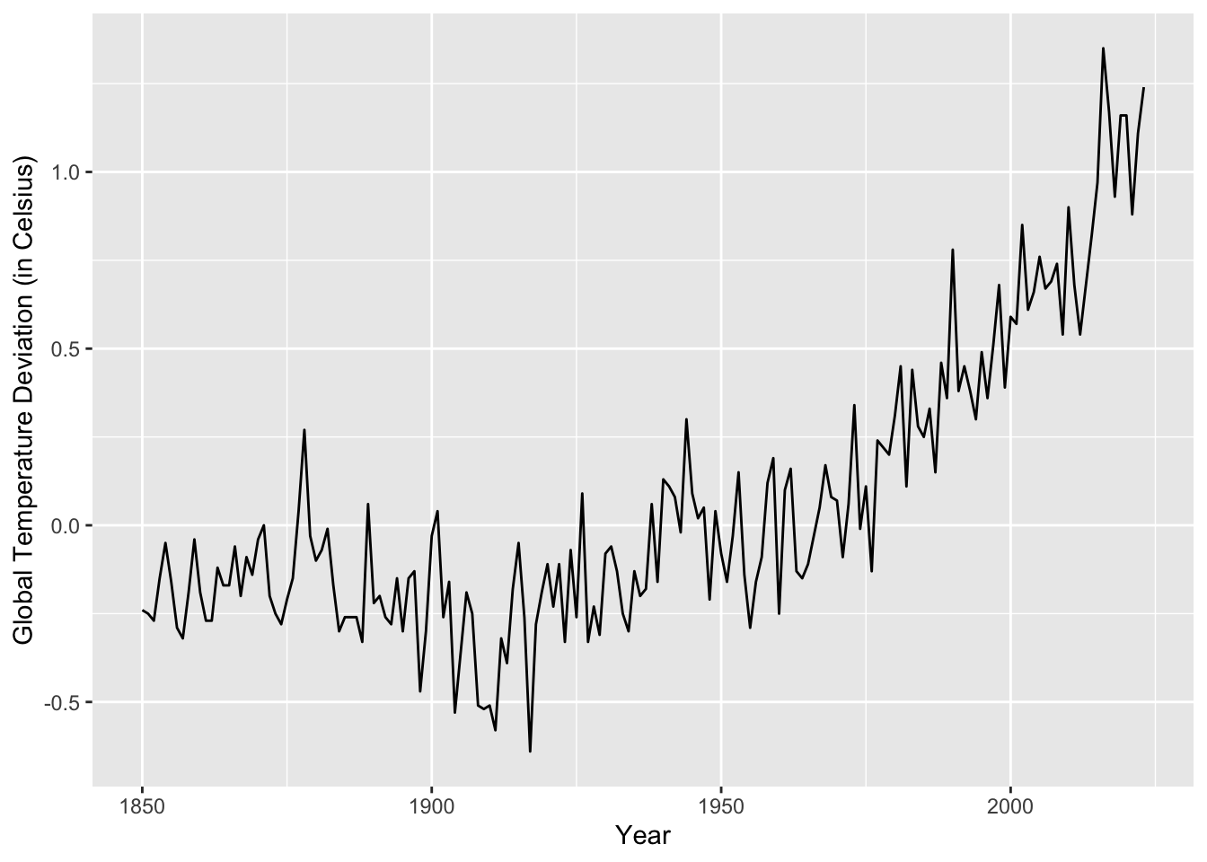
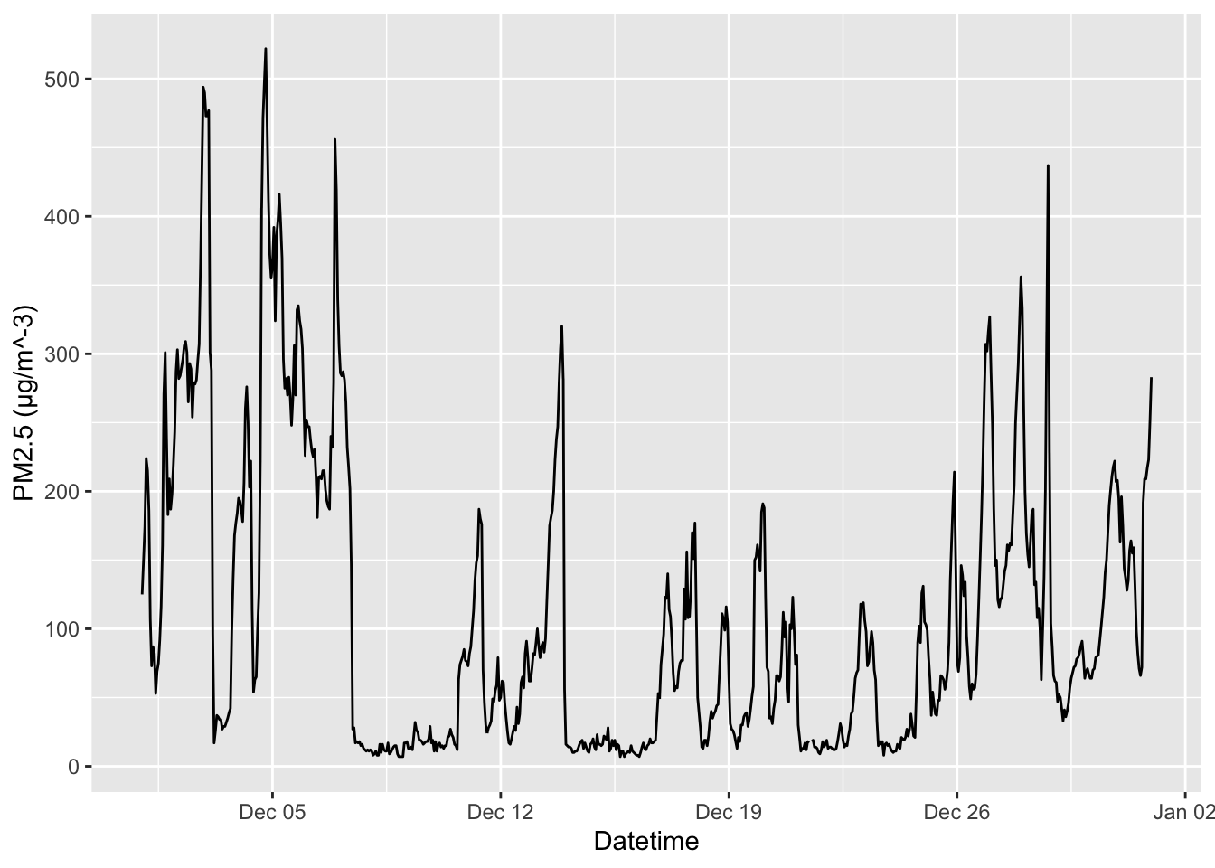
Climate change means that understanding the environment has never been more important. In environmental sciences, time series data are crucial to monitoring and understanding changes in environmental conditions, assessing the impact of human activities, and making informed decisions about environmental management. Such data include climactic measurements (temperature, precipitation, etc.), air quality, water quality, and biodiversity monitoring. In Figure 1.7, we plot the global yearly mean land–ocean temperature from 1880 to 2015, measured as deviations, in degrees Celsius, from the 1951-1980 average. ⁴ In Figure 1.8, we plot PM2.5 concentration levels in Beijing, measured hourly, in December 2011. ⁵

Figure 1.7: Global mean land–ocean temperature from 1880 to 2015, measured as deviations from the 1951-1980 average.

Figure 1.8: Hourly PM2.5 concentration levels in Beijing in December 2011.

1.2.5 Healthcare

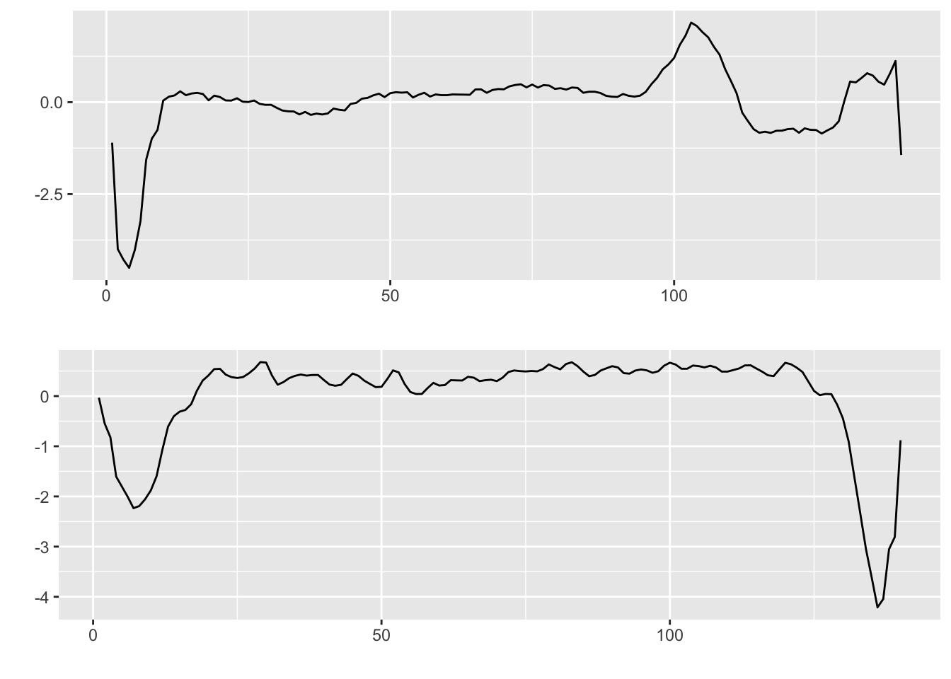
In 1901, Willem Einthoven invented the first practical electrocardiogram (ECG), which records the heart’s electrical activity (measured in terms of voltage) over time. ECGs can be used to diagnose cardiac abnormalities. In Figure 1.9, we show a portion of an ECG comprising a normal heartbeat (top), and a portion comprising an abnormal heartbeats. ⁶

Figure 1.9: The ECG recordings of two heartbeats from the same patient. The top panel records a normal heartbeat, while the bottom panel records an abnormal heartbeat.

More recently, the proliferation of sensors has led to the emergence of other time series data streams in healthcare data science. These include vital signs monitoring and data from wearable devices, and offer rich possibilities for innovations in patient diagnosis and treatment.

1.2.6 Physical sciences and engineering

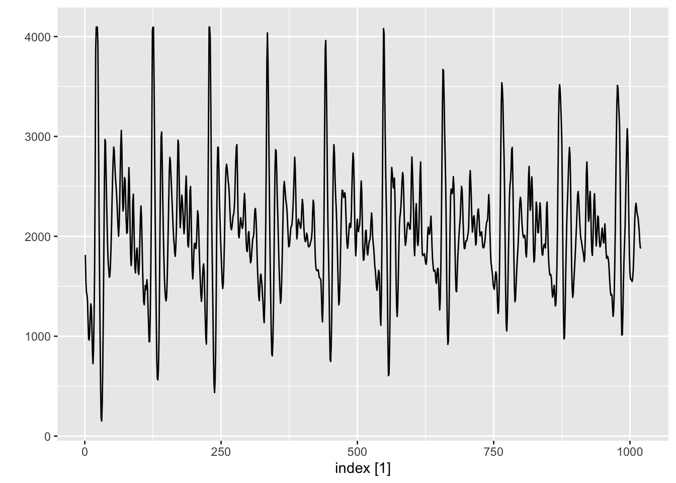
Time series data is also prevalent in the physical sciences and engineering. First, they arise when analyzing dynamical systems. For instance, the Apollo Project in the 1960s required estimation of the trajectories of spacecraft from noisy measurements as they traveled to the moon and back. They also occur when recording audio or taking measurements of other quantities using sensors. In Figure 1.10, we plot a 0.1 second segment of recorded speech for the phrase “aaahhhh”, sampled at 10,000 points per second.

Figure 1.10: A 0.1 second segment of recorded speech for the phrase “aaahhhh”, sampled at 10,000 points per second.

1.2.7 Comparison with “white noise”

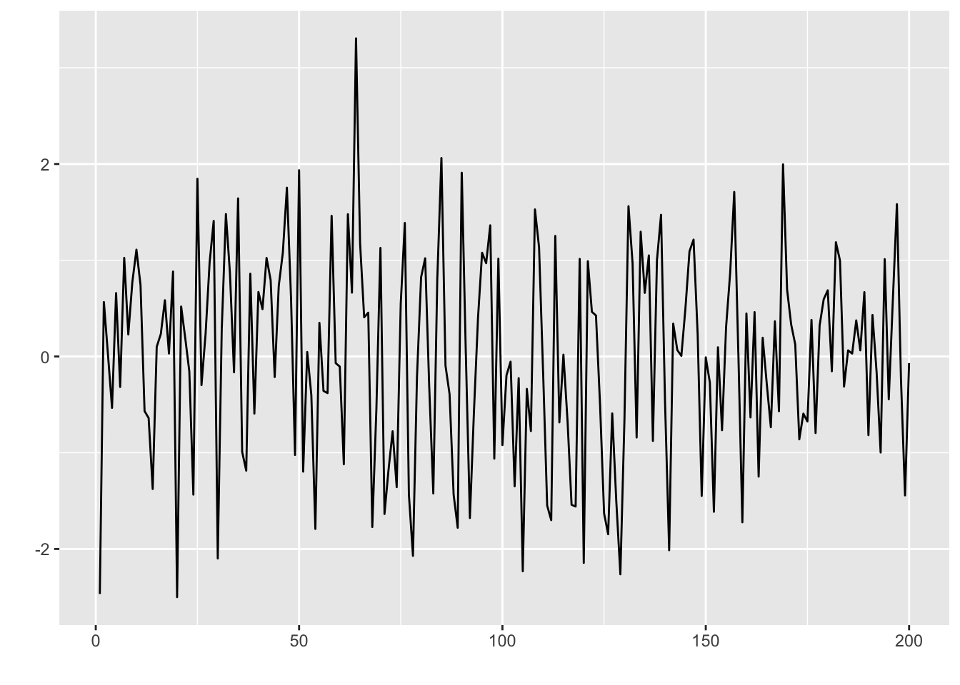
Even without any knowledge of time series analysis, several observations immediately stand out from the examples above. First is the sheer heterogeneity of time series data—the plots look very different from each other! Secondly, despite these differences, it seems apparent that most plots are not totally random, and some time-based structure can be extracted from them. To illustrate this, contrast the shape of their plots with that of “white noise” in Figure 1.11. White noise refers to a series of i.i.d. Gaussian measurements arranged in a sequence and thus has no structure at all.

Figure 1.11: White noise.

The overriding problem of time series analysis, and statistics in general, is how to extract signal from noise. We elaborate on this in the next subsection.

1.3 The goals of time series analysis

In this section, we will explore different categories of goals that researchers have when analyzing time series data.

1.3.1 Forecasting

One of the primary goals of time series analysis is forecasting. By analyzing historical data patterns, we can make predictions about future values. For instance, investment companies make profits based on their ability to forecast stock prices and volatility. Being able to forecast global mean temperature accurately allows scientists to more powerfully advocate for policies to mitigate climate change. On a shorter time scale, forecasting weather patterns allows us to plan our daily activities more effectively. Forecasting techniques range from simple methods like moving averages to more advanced models like ARIMA (AutoRegressive Integrated Moving Average) or machine learning algorithms.

1.3.2 Smoothing and filtering

Smoothing and filtering techniques are used to remove noise and extract underlying trends or patterns from time series data. These techniques help to reduce the impact of random fluctuations and highlight the long-term behavior of the data. For instance, during the Apollo Project in the 1960s, measurements obtained from spacecraft sensors were often noisy and subject to various disturbances. To extract the true position information from the noisy measurements, filtering techniques were employed. Methods used for smoothing and filtering have a large overlap with those used for forecasting.

1.3.3 Time series regression and adjustment

Time series regression involves modeling the relationship between a dependent variable and one or more independent variables, taking into account the time component. This allows us to analyze how the dependent variable changes over time and understand the impact of the independent variables on the time series. For instance, we might want to understand the effect of climactic factors on air pollution. Performing such a regression also allows to understand the impact of human intervention on air pollution by adjusting for different climactic conditions across different years.

1.3.4 Classification

Being able to tell the difference between the ECG of a normal heartbeat and an abnormal hearbeat allows us to diagnose cardiac abnormalities. More generally, in time series classification, we are given a collection of time series, where each time series is given a class label. The goal is to train a model to predict the label of unseen time series drawn from the same distribution. This is the same set-up as a regular classification problem, but the fact that each data point is a time series allows us to engineer time series features that may be much more predictive that the raw measurements.

1.4 Related problems*

Not all datasets with a time element are considered time series data. When measurements are taken continuously, or at irregularly spaced time intervals, then such data is more properly the domain of functional data analysis.

If the data arrives in a streaming fashion and actions taken at each time point can influence future measurements, then such a problem is analyzed using tools from reinforcement learning or control theory.

---

1. Data was obtained from https://finance.yahoo.com/quote/GOOG/.

2. Data was obtained from https://tablebuilder.singstat.gov.sg/table/TS/M212881.

3. Data was obtained from the fpp3 package associated with the textbook Hyndman, Rob J., and George Athanasopoulos. Forecasting: principles and practice. OTexts, 2018.

4. Data was obtained from the astsa package associated with the textbook Shumway, Robert H., David S. Stoffer, and David S. Stoffer. Time series analysis and its applications. Vol. 3. New York: Springer, 2000.

5. Data was obtained from https://www.kaggle.com/datasets/djhavera/beijing-pm25-data-data-set.

6. Data was obtained from https://www.timeseriesclassification.com/description.php?Dataset=ECG5000.