Appendix A — Background on R

A.1 Basics

A.1.1 Download and install

R is an open-source software for statistical computing. In our course, we shall use it along with the IDE Rstudio. You can download the two applications from here:

Note

Even if you already have R and Rstudio installed, please check and update them so that you have at least R >= 4.2 and Rstudio >= 2023.xx

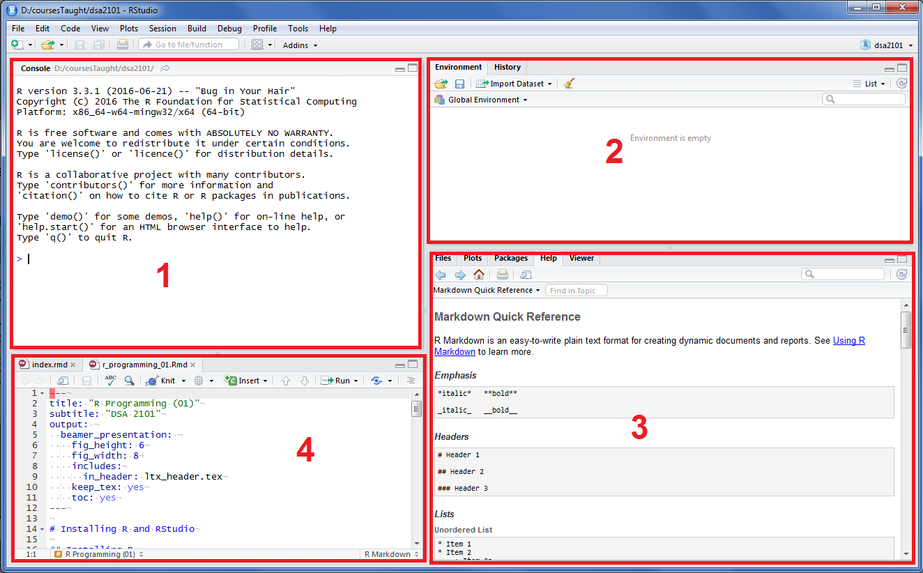
Although it can be reconfigured, the Rstudio interface typically consists of 4 sections:

Panel 1 is the console, where you type R commands. The output from commands also appears here.
Panel 2 contains the History and Environment tabs. Use these items to retrieve old commands and R objects created.
Panel 3 contains Files, Plots and Help tabs.
Panel 4 contains the source code editor. Edit R scripts and R markdown files here.

A.1.2 Vectors

R has no scalars. The basic building block for storing data in R is a vector. Vectors can be of different classes - typical classes are character, numeric, integer, logical and factor.

The following line creates a vector in R and then prints it out.

Z <- c(1, 2, 3)
Z

[1] 1 2 3

Elements in a vector are accessed using integers within the [ ] parentheses. Indices in R begin with 1 (not 0). Negative integers correspond to dropping those elements (not indexing from the end). Here are some examples:

X <- -2:2
Y <- 2^X

1Y[2]
2Y[2:4]
3Y[-c(3,5)]

1: Select 1st element from vector Y.
2: Select elements at positions 2, 3 and 4 from vector Y.
3: Drop elements at positions 3 and 5 from Y.

Note

In R, all elements in a vector must be of the same class.

A.1.3 Lists and Dataframes

Lists are collections of objects in R. The objects could be of different lengths and classes. To access elements within a list, use the $, [[ and [ operators.

ls1 <- list(A=seq(1, 5, by=2), B=seq(1, 5, length =4))

1ls1$A[2]
2ls1[["B"]][c(2,4)]
3ls1[[2]][c(2,4)]

1: Extract element 2 from A within the list.
2: Extract elements 2 and 4 from B within the list.
3: Extract elements 2 and 4 from B within the list, but using an integer within [[.

Warning

There are some subtle differences between [ and [[ but if you only use [[ when selecting an element from a list, and [ in all other cases, you should be alright.

In R, a data frame is a special kind of list. A data frame is a tabular object that is used to store data. The columns can be of different class.

1exp_cat <- c("manpower", "asset", "other")
amount <- c(519.4 , 38, 141.4)
2op_budget <- data.frame(amount, exp_cat)

1: Create two vectors (one of class character and another numeric).
2: Combine them into a data frame.

The data frame is like a table:

amount	exp_cat
519.4	manpower
38.0	asset
141.4	other

Just like a list, elements in a data frame can be accessed using $ and [. However, since the data frame is two-dimensional, we need two indices when we use [.

1op_budget$amount
2op_budget[, "exp_cat"]
3op_budget[c(3,2), ]

1: Retreive amount column.
2: Retreive exp_cat column.
3: Retrieve rows 3 and 2 (in that order) from the data frame.

A.1.4 Functions and Arguments

We have already encountered a few functions in R: list(), data.frame() and seq(). Functions in R have arguments. To get help on any function, use this command:

?data.frame

This will pull up the help page for that particular function (no internet needed). All arguments will be documented, along with working examples right at the bottom.

Here is a list of common R functions that will be handy to know:

Command	Description
`read.csv()`	Used to read data from CSV files.
`head()`	Displays the first few rows of a data frame.
`tail()`	Displays the last few rows of a data frame.
`summary()`	Provides 5-number summary for a data frame.
`ls()`	List the objects in the current R workspace.
`length()`	Find the length of a vector.
`seq()`	Generate a regular sequence of numbers.
`mean()`,`median()`	Compute the mean,median of a vector.
`sd()`,`var()`	Compute the sd,var of a vector.
`+`, `-`, `*`, `/`, `^`	Basic arithmetic binary operators.
`==`, `!=`, `>`, `<`, `>=`, `<=`	Logical comparisons (return logical vector).

A.1.5 Installing Packages

There are numerous packages that can be installed to extend the functionality of R.

A package is simply a collection of functions.

Most R packages are hosted on CRAN. At my last check, there were 19880 packages. There is also a sizeable number on bioconductor and on github.

Before using a package, we need to install it. This only needs to be done once. Here is the command to install a package named stringr:

install.packages("stringr")

Every time we start an R session, we have to load the package(s) that we wish to use before we can call functions from it.

library(stringr)

A.2 Tidyverse and Piping

A.2.1 Tidyverse

The tidyverse refers to a set of R packages that implement routines that make it easier to manipulate data. They are based on the concept of tidy data.

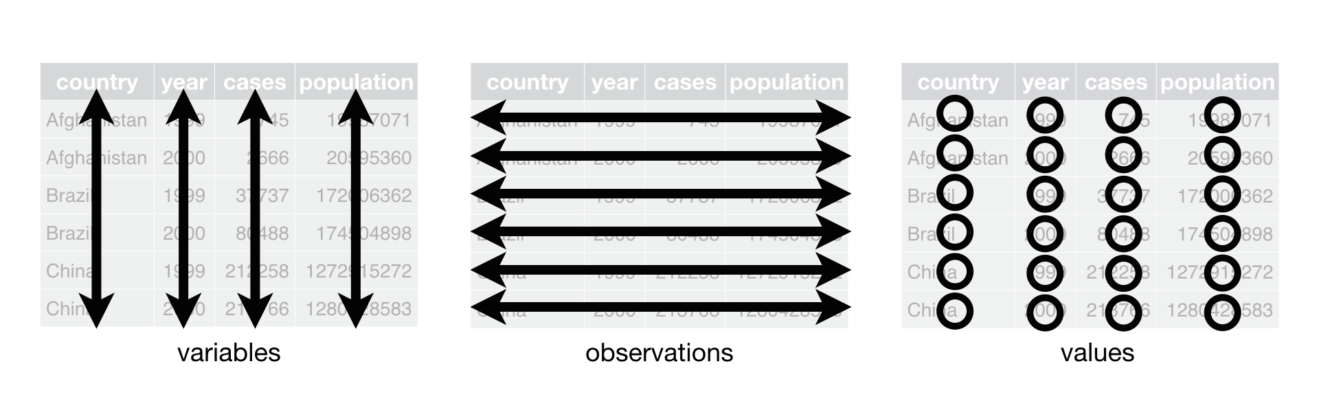
Tidy data requires that

Each variable forms a column.
Each observation forms a row.
Each type of observational unit forms a table.

The following command loads the tidyverse set of packages. You will observe several warnings regarding conflicts, but it’s ok to proceed in this case.

library(tidyverse)

The R packages that we are going to use for forecasting use the tidyverse extensively. Hence it is important for us to learn about the tidyverse. It does indeed take a little time to get used to, but once you are comfortable, it is quite intuitive to work with.

A.2.2 Tibbles

A tibble is an object designed by the creators of the tidyverse. It is different from data frames in a few ways. The most noticeable differences are:

When printing, it does not print all rows and columns. This makes it better for inspecting a data frame.
The variable types are shown, and numerical values are colour-coded and rounded for easier visual scanning.

This is the output when printing a tibble in R:

cars_tbl <- as_tibble(cars)
cars_tbl

# A tibble: 50 × 2
   speed  dist
   <dbl> <dbl>
 1     4     2
 2     4    10
 3     7     4
 4     7    22
 5     8    16
 6     9    10
 7    10    18
 8    10    26
 9    10    34
10    11    17
# ℹ 40 more rows

The output from printing a raw data frame in R is much more verbose. In this case, printing cars would display all 50 rows.

A.2.3 Basic Data Manipulation Verbs

There are many functions from the dplyr package within the tidyverse that make data manipulation.. fun! Here are couple that we will be using quite often.

The filter() function keeps only rows whose columns satisfy certain criteria. The criteria are specified as logical vectors after the dataframe.

mtcars_tbl <- as_tibble(mtcars)
filter(mtcars_tbl, cyl <= 4)

# A tibble: 11 × 11
     mpg   cyl  disp    hp  drat    wt  qsec    vs    am  gear  carb
   <dbl> <dbl> <dbl> <dbl> <dbl> <dbl> <dbl> <dbl> <dbl> <dbl> <dbl>
 1  22.8     4 108      93  3.85  2.32  18.6     1     1     4     1
 2  24.4     4 147.     62  3.69  3.19  20       1     0     4     2
 3  22.8     4 141.     95  3.92  3.15  22.9     1     0     4     2
 4  32.4     4  78.7    66  4.08  2.2   19.5     1     1     4     1
 5  30.4     4  75.7    52  4.93  1.62  18.5     1     1     4     2
 6  33.9     4  71.1    65  4.22  1.84  19.9     1     1     4     1
 7  21.5     4 120.     97  3.7   2.46  20.0     1     0     3     1
 8  27.3     4  79      66  4.08  1.94  18.9     1     1     4     1
 9  26       4 120.     91  4.43  2.14  16.7     0     1     5     2
10  30.4     4  95.1   113  3.77  1.51  16.9     1     1     5     2
11  21.4     4 121     109  4.11  2.78  18.6     1     1     4     2

filter(mtcars_tbl, cyl <= 4, vs == 0)

# A tibble: 1 × 11
    mpg   cyl  disp    hp  drat    wt  qsec    vs    am  gear  carb
  <dbl> <dbl> <dbl> <dbl> <dbl> <dbl> <dbl> <dbl> <dbl> <dbl> <dbl>
1    26     4  120.    91  4.43  2.14  16.7     0     1     5     2

The select() function selects only the columns specified. The specification of columns is very flexible. See ?select for more examples.

1select(mtcars_tbl, mpg:hp)
2select(mtcars_tbl, !c(mpg:hp))
3select(mtcars_tbl, last_col(offset=1):last_col())

1: Select all columns from mpg to hp.
2: Select all columns except mpg to hp.
3: Select the last two columns.

Note

Observe that we do not need to quote the column names! We can just type mpg in the expression instead of "mpg". This saves typing in interactive analysis.

Note

Most dplyr verbs have a common syntax:

data_frame <- fn_name(data, verb-specific-1, verb-specific-2,...)

The verbs work with data frames too, but as we know, tibbles print nicer!

A.2.4 Piping

Another practice that the tidyverse popularised was the use of the pipe operator.

Manipulating data typically involves many steps, and using a pipe operator allows us to daisy chain operations while retaining readable code. In R, the pipe operator %>% from the magrittr package unwraps:

x %>% f(y) into f(x,y), and
x %>% f(y) %>% g(z) into f(x,y) %>% g(z), which is just g(f(x,y), z)

Suppose we wish to combine the filter and select operations from earlier. Without the pipe operator, we would do one of the following:

# Method 1
select(filter(mtcars_tbl, cyl <= 4, vs == 0), mpg:hp)

# Method 2
tmp <- filter(mtcars_tbl, cyl <= 4, vs == 0)
select(tmp, mpg:hp)

But with the piping approach, we just need:

mtcars_tbl %>%  
  filter(cyl <= 4) %>%  
  select(mpg:hp)

A.3 ggplot

ggplot2 implements the grammar of graphics, which is a method of building up graphics from components. It uses an approach that centers around layers.

The following code will create a plot, placing mpg variable on the y-axis and disp on the x-axis.

1ggplot(mtcars_tbl) +
2  geom_point(mapping=aes(x=disp, y=mpg))

1: The first layer ggplot( ) has to specify the dataset. The + operation adds layers to the plot. Layers could be another set of points, a label for the legend or a title, or a specification of symbol types.
2: geom_point summons a scatterplot. Other geoms that might be useful are:

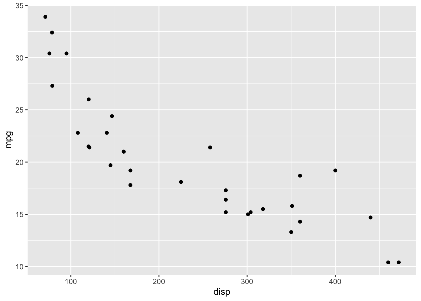
Perhaps the most confusing aspect of ggplot is the “mapping”. A graph is a visualisation of the variation of numbers in a dataset. When we construct a graph, we can view it as a process of choosing colours, positions, shapes, and/or lengths to vary according to the data. This mapping is what we explicitly provide to a ggplot call.

In the above case, we mapped the disp variable to positions on the x-axis and the mpg variable to positions on the y-axis.

In our course, the packages we are going to rely on also use ggplot2 to make plots. Most of the time, we can simply call autoplot() on our time series objects, but having a basic grasp of how ggplot2 works will be useful.

A.4 R Markdown

A.4.1 Background

R Markdown is a scripting language that allows you to combine code, its results and your text into one text document. That text document can then be “knitted” into a range of output formats, including html, pdf and Word.

Because it is just a text document, R Markdown is very useful when you wish to create work/analysis that can be reproduced and extended by others. Also because it is essentially just a text document, it can be version-controlled easily.

Note that there are many “flavours” of Markdown, including github, R, obsidian, etc.

A.4.2 Basics

The first section of an Rmd file is usually a YAML header, surrounded by —s. YAML stands for Yet Another Markup Language. We will usually not have to write this ourselves. The Rstudio IDE takes care of this. It will look like this:

---
title :  "Diamond sizes"
date : 2023 -08 -25
output : html_document
---

The rest of the document consist of code chunks (R code) and formatted text. The code chunks are defined with three tick-marks:

```{r}
# Write your R code here
```

The text that you write will be formatted with #, * and other Markdown operators. If you are familiar with HTML, then Markdown will come easily, as it is in fact just another markup language.

A.5 Additional References

Wickham, H., Çetinkaya-Rundel, M., & Grolemund, G. (2023). R for data science. ” O’Reilly Media, Inc.”.
Posit cheatsheets:
ggplot2 documentation page: This page contains further links to useful articles, books and galleries.
Original specification of Markdown
Project structure: Some tips on naming conventions and folder structure for effective workflows.
Further resources on learning R:
- Use your DataCamp accountto go through the courses you need.
- Use chatGPT to help you understand or debug code.