In Chapter 3, we learnt about three time series patterns: trend, seasonality, and cycles. We saw in that chapter how to visualize and identify these patterns using visualizations. In Chapter 4, we learnt about how to apply transformations to extract patterns from time series. The idea of time series decomposition emerges from the combination of these ideas.
We start with the belief that a time series \((x_t)\) can be written as \[
x_t = T_t + S_t + R_t,
\tag{5.1}\] where \(T_t\) is a slowly changing trend-cycle component, \(S_t\) is a seasonal component, and \(R_t\) is an irregular remainder term. Trend and seasonality are captured by the first two terms, while cycles are divided between \(T_t\) and \(R_t\) depending on their frequency. \(R_t\) also contains everything else about the time series that cannot be explained by the other two components. It is also called the random or noise component. While there is no a priori reason why any time series \((x_t)\) satisfies such a decomposition, it seems to be a reasonable assumption for many real world time series.
Next, given this belief, we would like to find transformations of \(x_t\) that allow us to extract \(T_t\), \(S_t\), and \(R_t\). There are multiple versions of such transformations, and we will discuss some of these in this chapter.
Decomposing the time series allows us to understand it better, as the individual components may have meaning for analysts. We can visualize them and use them to compute useful summary statistics. It can also help with forecasting. Analysts also sometimes wish to remove one component to focus on the other components. If the trend component is removed, we say that the resulting time series detrended, if the seasonal component is removed, we call the resulting time series seasonally adjusted.
5.2 Classical decomposition
The classical decomposition makes some further assumptions in addition to Equation 5.1. First, \(T_t\) and \(S_t\) are treated as deterministic, while \(R_t\) is modeled as a mean zero stationary stochastic process. We discuss stationarity more rigorously in Part 2 of this book, but for now, this implies that the mean of an increasing number of observations of \(R_t\) tends to 0, i.e. for any \(t\), \[
\frac{1}{m}\sum_{j=1}^{m}R_{i_j} \to 0
\tag{5.2}\] in probability as \(m \to \infty\), for any sequence of indices \(i_1, i_2,\ldots\). Furthermore, we assume that the seasonality is constant, i.e. if the period of the seasonality is \(p\), then we have \[
S_{t+p} = S_t
\tag{5.3}\] for any time \(t\). For identifiability reasons, we also assume that \[
\frac{1}{p}\sum_{j=0}^{p-1} S_{t+j} = 0,
\tag{5.4}\] or in other words, that \(S_t\) has mean zero across the time series.
These assumptions allow us to estimate \(T_t\), \(S_t\) and \(R_t\) as follows. Assuming that \(k+l+1\) is a multiple of the period \(p\), we can estimate the trend-cycle component via: \[
\frac{1}{m}\sum_{j=-k}^l x_{t+j} = \underbrace{\frac{1}{m}\sum_{j=-k}^l T_{t+j}}_{\approx T_t} + \underbrace{\frac{1}{m}\sum_{j=-k}^l S_{t+j}}_{= 0} + \underbrace{\frac{1}{m}\sum_{j=-k}^l R_{t+j}}_{\approx 0} \\
\] Here, the first term is approximately \(T_t\) because of the slowly-changing nature of the trend-cycle component, the second term is zero because of Equation 5.4, while the last term is approximately zero because of Equation 5.2.
Meanwhile, for any \(1 \leq k \leq p\), the detrended time series \(x_t - T_t\) satisfies: \[
\frac{1}{m+1}\sum_{j=0}^m \left(x_{k + jp} - T_{k + jp} \right) = \underbrace{\frac{1}{m+1}\sum_{j=0}^m S_{k + jp}}_{= S_k} + \underbrace{\frac{1}{m+1}\sum_{j=0}^m R_{k + jp}}_{\to 0}
\tag{5.5}\] as \(m \to \infty\). The first term is equal to \(S_k\) because of Equation 5.3, while the second term tends to 0 by Equation 5.2. This allows us to estimate the seasonal component, and we obtain the remainder by subtracting both our estimates of \(T_t\) and \(S_t\) from \(x_t\).
We can summarize this as the following algorithm.
Step 1: Compute an estimate \(\hat T_t\) for \(T_t\) by taking a moving average of window size \(p\) or \(2p\), where \(p\) is the period of the seasonality.
Step 2: Take the mean over the detrended series, \(x_t - \hat T_t\) over all time indices with the same season (e.g. all March months for monthly time series with yearly seasonality) to get an an estimate \(\hat S_t\) for the seasonal component for that season.
Step 3: Estimate the remainder via \(\hat R_t = x_t - \hat T_t - \hat S_t\).
5.3 Multiplicative decomposition
When the amplitude of the fluctuations (seasonality, cycles) increase with the level of the time series, it may be more reasonable to believe in a multiplicative decomposition rather than an additive one. A multiplicative decomposition takes the form \[
x_t = T_t \cdot S_t \cdot R_t,
\] where \(T_t\), \(S_t\), and \(R_t\) have the same meanings as before. We can turn this into an additive decomposition by taking logarithms: \[
\log x_t = \log T_t + \log S_t + \log R_t
\] after which we can estimate each component via classical decomposition as before.
5.4 Some examples
To illustrate the use of classical decomposition, let us apply it to the aus_arrivals dataset comprising tourist arrivals to Australia.
aus_arrivals |>filter(Origin =="UK") |>1model(classical_decomposition(Arrivals, type ="multiplicative")2 ) |>3components() |>4autoplot()
1
model() is a function from the fabletools package that trains a model.1
2
Here, we have selected the classical_decomposition() model and selected the type of decomposition to be multiplicative (rather than additive).
3
components() is a generic function that extracts the components from the fitted model.
4
autoplot() is applied directly to the object returned by components() and knows to automatically produce the faceted time plots shown below.
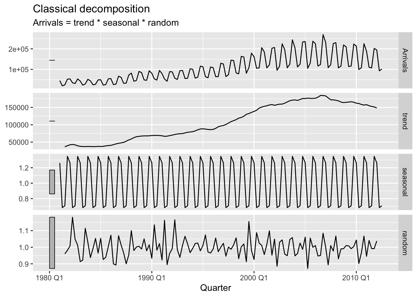
Figure 5.1: Tourist arrivals to Australia from the UK.
Here, we have used a multiplicative decomposition, which seems more appropriate after inspecting the time plot of the original time series. The trend component displays an increasing trend, which plateaus around 2005. The seasonal component displays the seasonality which is high in Q1 and Q4 (Summer) and low in Q2 and Q3 (Winter). The decomposition allows us to be even more precise: In Q4, the tourist arrivals are almost 40% higher than average, while in Q2, they are only 70% of the average. Finally, the remainder component does not illustrate any systematic patterns or trend, and is instead centered at the value 1 (recall that the decomposition is multiplicative). This indicates that the assumptions of the classical decomposition are reasonable for this time series.
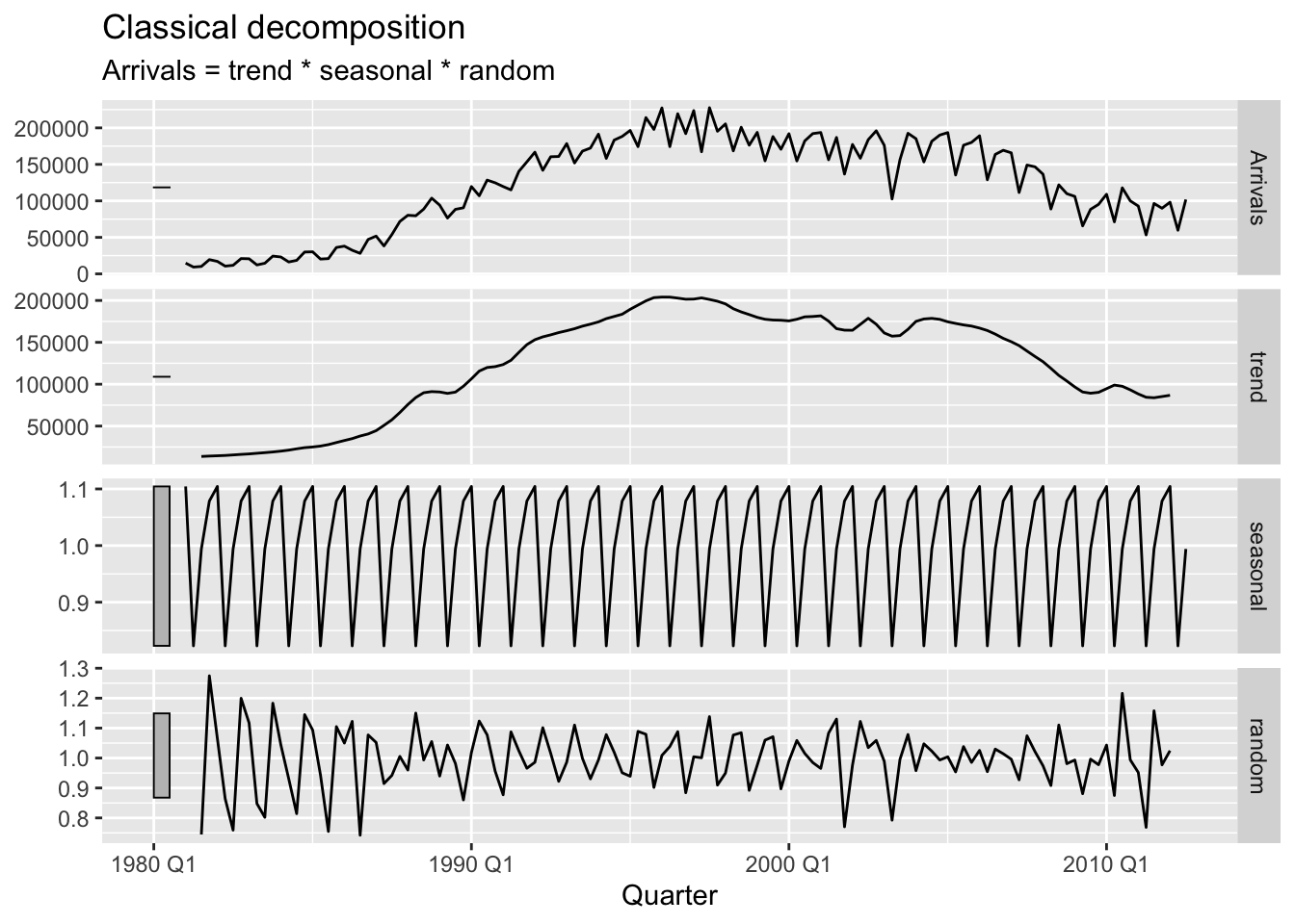
We next apply a multiplicative decomposition to the arrivals from Japan. The results are shown in Figure 5.2.
Figure 5.2: Tourist arrivals to Australia from Japan.
In comparison with Figure 5.1, the remainder component displays some troubling patterns. First, its fluctuations seem to be heteroscedastic—they are larger prior to 1988 than afterwards. Second, it also seems to contain a regular repeating pattern prior to 1988. In sum, the fitted remainder component does not seem stationary, contrary to the assumptions of classical decomposition. To explain, recall our discussion in Chapter 3 that the seasonality for this time series changes around 1995 (see also Figure 3.3.) On the other hand, classical decomposition assumes that the seasonality remains constant (Equation 5.3).
5.5 Advanced decompositions
Classical decomposition suffers from several notable problems. First, it assumes that the seasonality remains constant (Equation 5.3), which is not always a reasonable assumption, as evidenced by Figure 5.2. Moreover, it is overly sensitive to particularly unusual values (i.e. outliers), such as the period when there were no passengers in 1989 in Figure 1.6 because of a strike. Other issues are discussed in Chapter 3.4 of Hyndman and Athanasopoulos (2018).
New decomposition approaches have been developed to address these issues. Here, we briefly introduce the STL decomposition method, which stands for Seasonal and Trend decomposition using Loess (Cleveland et al. (1990)). Loess is a method for nonparametric smoothing, and is used repeatedly in STL. The algorithmic details of STL and other advanced decomposition approaches remain out of the scope of this textbook (and course.) We refer the interested reader to Hyndman and Athanasopoulos (2018).
We call the STL() function to fit our model. Note that the syntax resembles that for lm().2
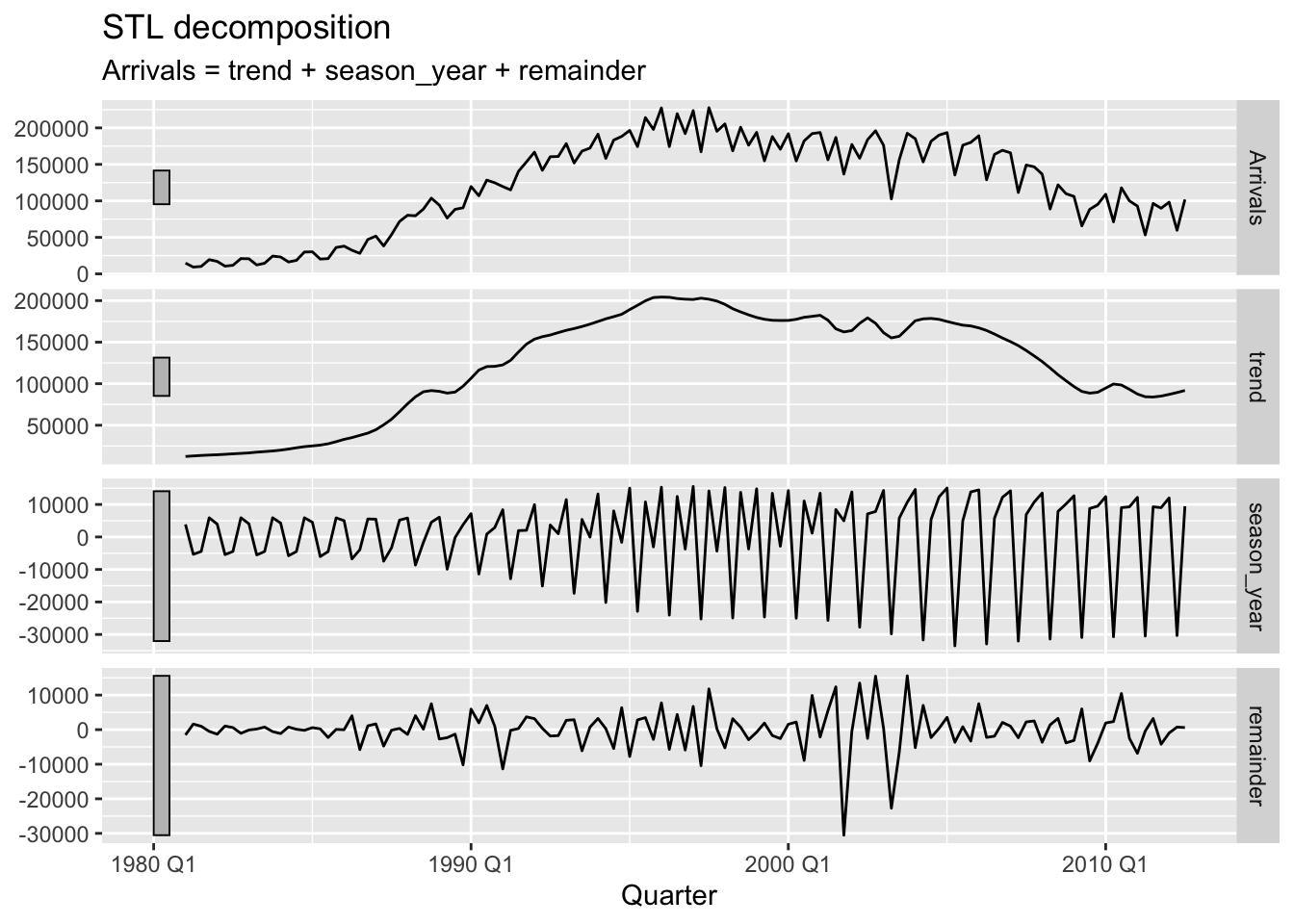
Figure 5.3: Tourist arrivals to Australia from Japan.
In comparison with Figure 5.2, Figure 5.3 clearly shows that the yearly seasonality is changing over time. The shape of the trend remains roughly the same, while the remainder component now does not display any regular patterns.
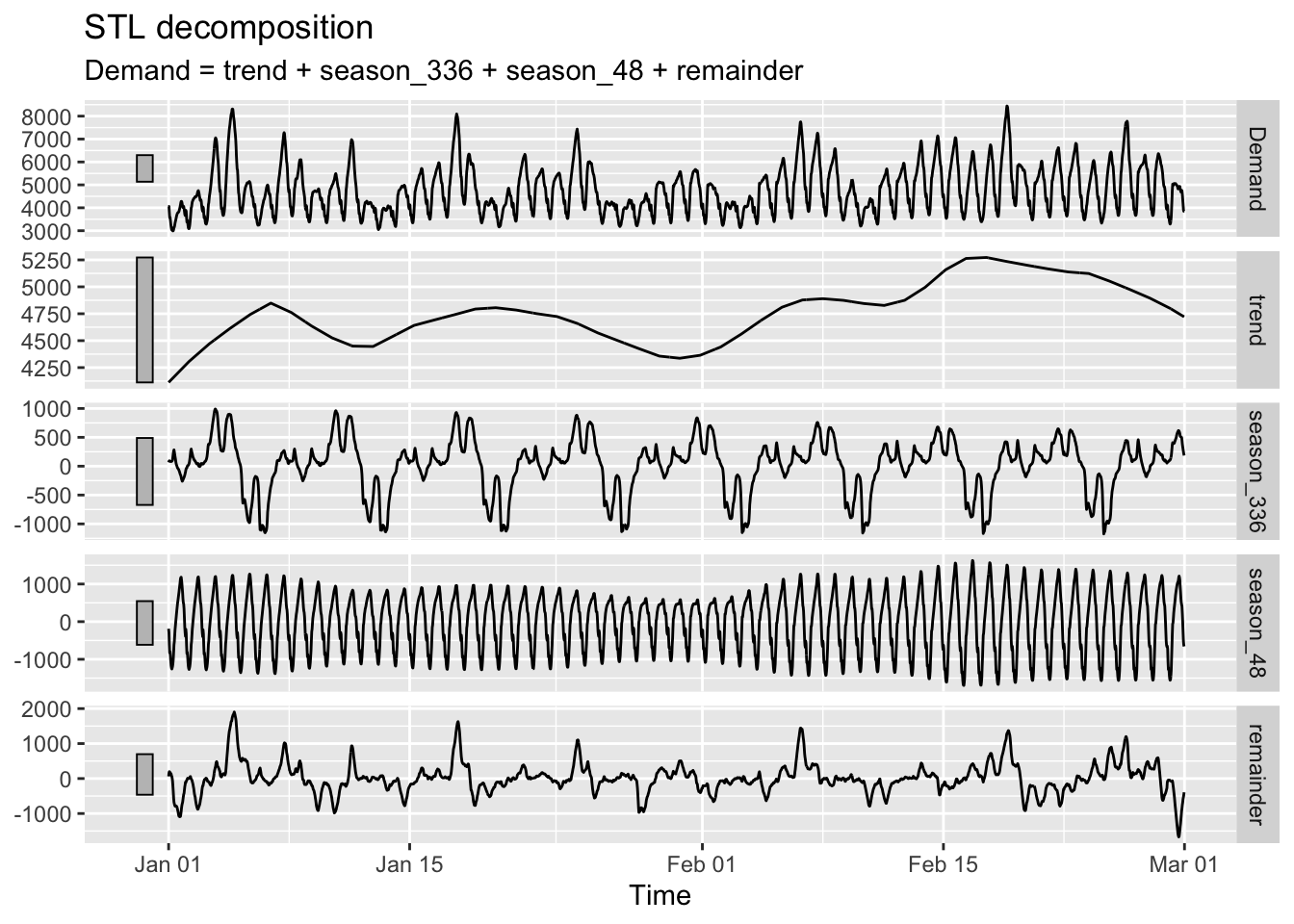
We next decompose vic_elec, which records energy consumption in Victoria, Australia. As shown in Chapter 2.4 of Hyndman and Athanasopoulos (2018), this time series displays multiple seasonality. The STL decomposition is able to extract multiple seasonal components as follows.
We set the period of one seasonal componet to be 48 * 7 to extract the weekly seasonality.
2
We set the period of the second seasonal component to be 48 to extract the daily seasonality.
Figure 5.4: Energy demand in Victoria, Australia in January and February 2013, measured half-hourly.
Reading the \(y\)-axis tick labels allows us to compare the scale of the different components. We see that the daily seasonal component is larger than that of the weekly component. If no period argument is supplied to season(), the seasonal periods are estimated automatically.
Cleveland, Robert B, William S Cleveland, Jean E McRae, and Irma Terpenning. 1990. “STL: A Seasonal-Trend Decomposition.”J. Off. Stat 6 (1): 3–73.
Hyndman, Rob J, and George Athanasopoulos. 2018. Forecasting: Principles and Practice. OTexts.
We will discuss the functions and data structures used here in more detail in Chapter 6.↩︎
The window size used for smoothing the trend and seasonal components can be adjusted via setting the window argument of trend() and season().↩︎