library(fpp3)
library(tidyverse)
library(gridExtra)3 Visualizations
Before performing modeling with data, one ought to first perform exploratory data analysis. A big part of this is creating helpful visualizations and using them to guide further analysis. In this section, we will learn how to create several types of plots.
These plots can be used to identify patterns or characteristics of the time series data. For instance, we can identify whether the time series possesses one (or more) of the following patterns:
- Trend: A long term increase or decrease.
- Seasonality: A pattern that recurs at regularly spaced intervals.
- Cycles: Repeated rise and falls that do not occur at regular intervals. These are associated with certain types of autoregressive behavior, which we will discuss more rigorously in the next part of the book.
Note
Understanding what patterns are present in the time series data can help to guide us in deciding what model to fit to the data, or to inspect models that have already been fit.
Of course, identifying a given pattern as a trend, seasonality, or cycle is sometimes more heuristic than rigorous. It may also depend on the observed time scale. For instance, some of the initial debate about climate change was whether the observed increase in temperatures was part of a trend or a very long-term naturally-occuring cycle.
As you follow along in this chapter, make sure the following packages are loaded:
3.1 Time plots
The time plot is the most natural first thing to do with a time series. It plots the measurements on the y-axis, time on the x-axis and joins the points together with a line. We have already seen a number of time plots in a previous section.
Generating a time plot from a tsibble is incredibly easy via autoplot().
aus_airpassengers |>
    autoplot(.vars = Passengers) +
    geom_point() +
    labs(y = "Passengers (millions)",
         x = "Year")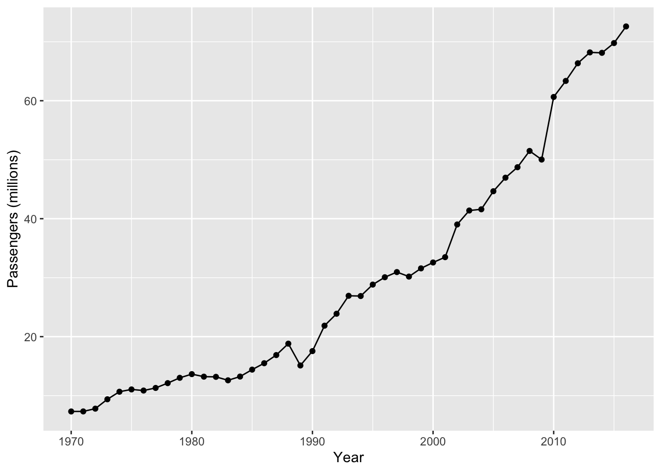
There is a general upward trend of passengers. There were two noticeable dips—one in 1989 and one in 2009 (what happened?). It is arguable that the trend appears piecewise linear, with a more positive gradient after 1990.
When the tsibble contains multiple time series, autoplot() makes a line plot for each of them, i.e. the number of lines is the number of unique keys. This can easily lead to overplotting (see Figure 1.4), so one is advised to first filter for only the most relevant keys before plotting.
Let’s look at another time plot, which shows the quarterly arrivals of tourists to Australia from Japan.
aus_arrivals |> filter(Origin=="Japan") %>%
  autoplot(.vars=Arrivals)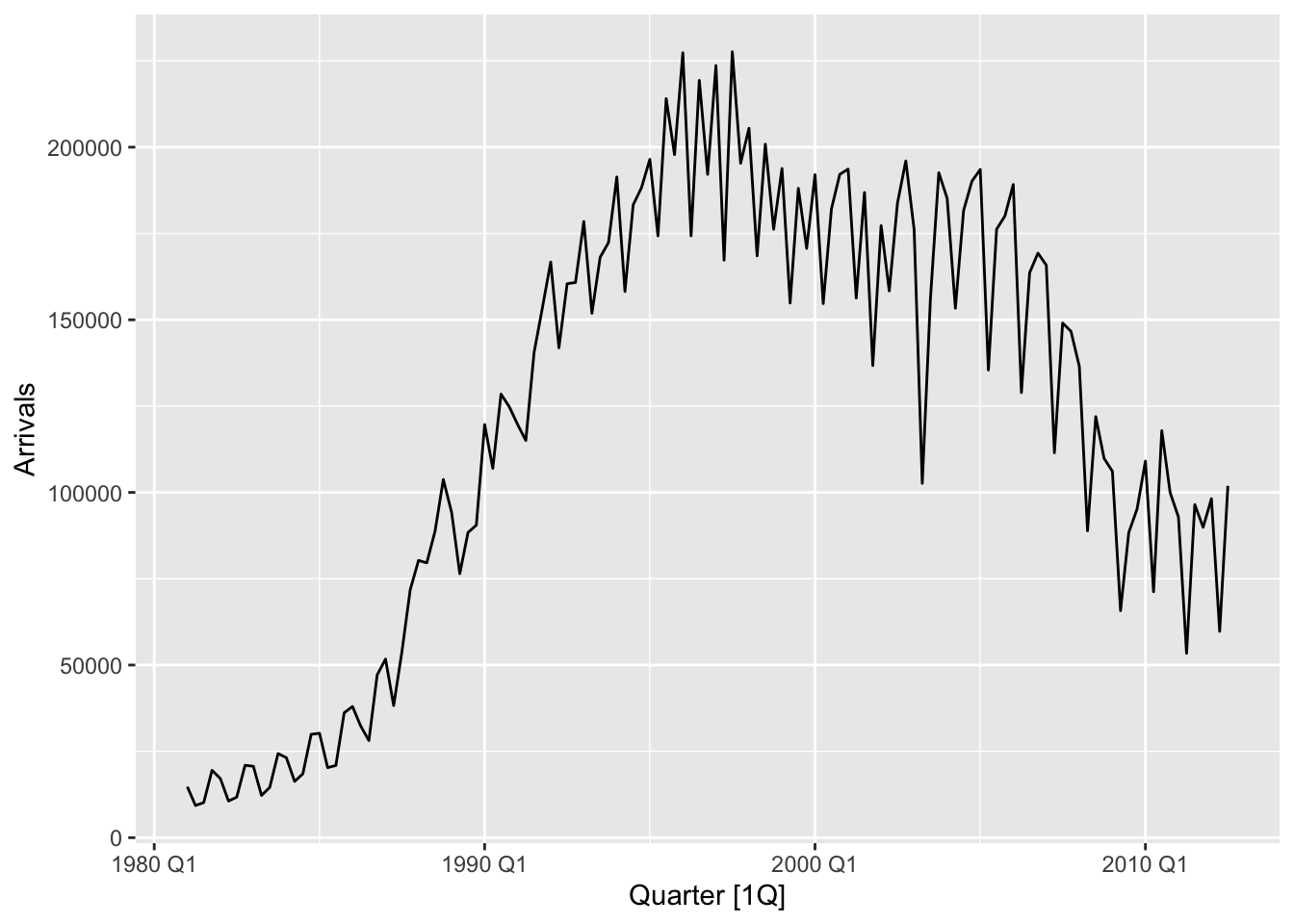
There was a strong upward trend until around 1995. Since then the arrivals has been decreasing (Why?). There is a sharp dip in arrivals (compared to neigbouring quarters) in 2003 Q2. The seasonal effect is strong throughout, but it became more regular after 1995.
Note how we have discussed the time plots in Figure 3.1 and Figure 3.2. Time plots are arguably most useful for detecting trends. While they can also be used to detect seasonality and cycles, these patterns can be made more apparent by other types of plots.
3.2 Seasonal plots
We first introduce some terminology for talking about seasonality. The period of a seasonality is the number of time units before the pattern repeats itself. 1 A season is a particular phase of the repeated unit. When the time series is quarterly and the period is a year, this corresponds to Spring, Summer, Fall, and Winter. More generally, there is one season for every time unit until the pattern repeats itself.
A seasonal plot is similar to a time plot, except that we chop up the time series into period lengths, align these pieces, and plot them on the same axes. We now make such a plot for the the data on arrivals to Australia from Japan, first dividing the time series into the portion before the start of 1995 and the portion after it.
plt1 <- aus_arrivals |>
    filter(Origin == "Japan", Quarter <= yearquarter("1995 Q4")) |>
    gg_season(y = Arrivals, labels = "right") +
    lims(y=c(9000, 230000))

plt2 <- aus_arrivals |>
    filter(Origin == "Japan", Quarter > yearquarter("1995 Q4")) |>
    gg_season(y = Arrivals, labels = "right") +
    lims(y=c(9000, 230000))

grid.arrange(plt1, plt2, nrow = 2)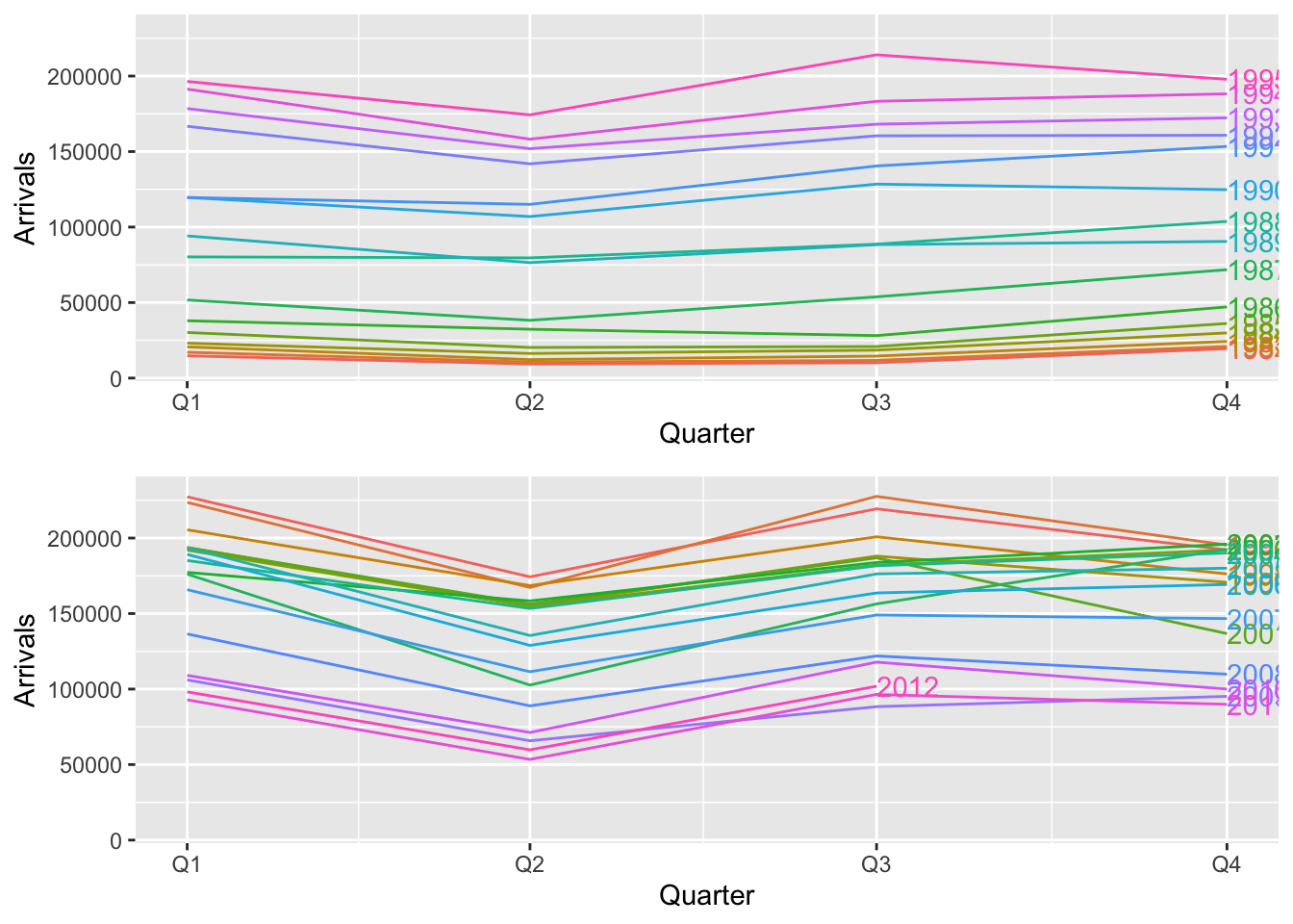
Notice that we did not have to tell gg_season() what the period of the seasonality was—it was automatically estimated from the data. This plot reveals the yearly seasonality more clearly, and shows that the pattern becomes more regular after 1995. Furthermore, the precise pattern becomes obvious. For instance, we can easily tell that the arrivals in Q2 is generally lower than the other quarters. Furthermore, we can pick out the trend more easily. Note that the year that each line corresponds to is indicated on the right of the line. In the top panel, lines correspond to earlier years as we go down the y-axis. In the bottom panel, going down corresponds to more recent years. This reflects the change in trend.
Many time series have seasonalities of multiple periods. We can choose what period to use for gg_season() by setting the period argument, e.g. to “day”, “week”, or “year”. For instance, consider the dataset vic_elec, which measures the half-hourly electricity demand for the state of Victoria in Australia. The seasonal plots corresponding to these periods are shown in Chapter 2.4 of Hyndman and Athanasopoulos (2018).
3.3 Seasonal subseries plots
A seasonal subseries plot stratifies the data according to the season and then makes a separate time plot for each season. 2 We again make a plot using the data on arrivals to Australia from Japan.
aus_arrivals |> filter(Origin == "Japan") %>%
  gg_subseries(y = Arrivals)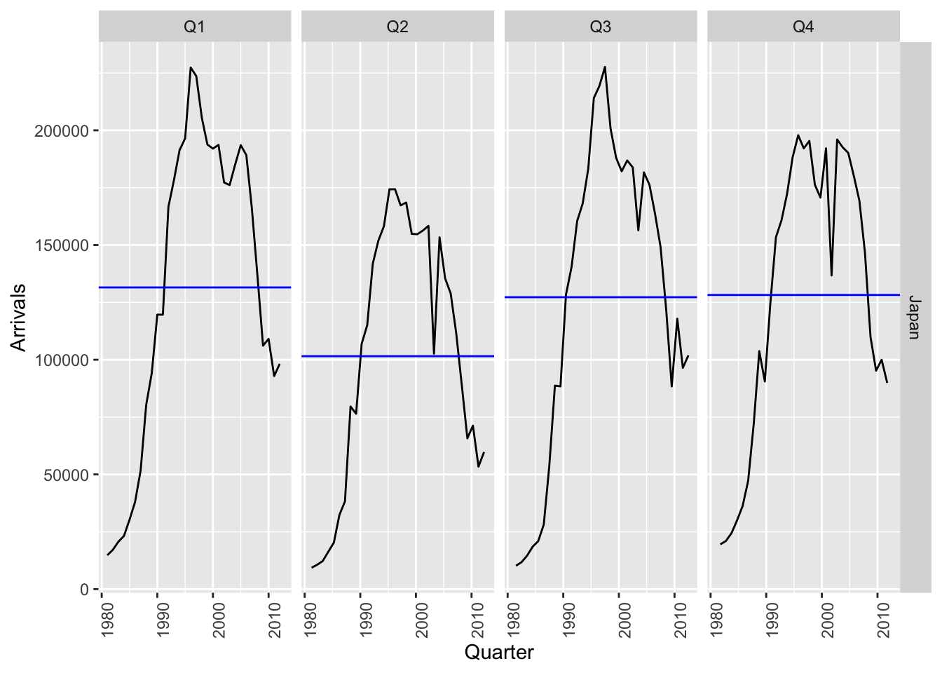
This plot shows the trend very clearly, as well as that it is relatively independent of the season. Note that the blue horizon line in each subplot shows the mean of the data for that quarter.
3.4 Scatter plots
As described in the previous section, tsibbles can contain multiple time series. This can be because a key variable is present, or because the time series data is multivariate (i.e. measures multiple types of quantities across the same duration of time). When we want to study the relationships between multiple time series, we may use scatterplots, just like we would in studying the relationships between different features in non time series data.
Let us make a pairs plot for the tourist arrivals to Australia from four different regions, contained in aus_arrivals.
library(GGally)
pivot_wider(aus_arrivals, names_from = "Origin", values_from="Arrivals") |>
  ggpairs(columns=2:5)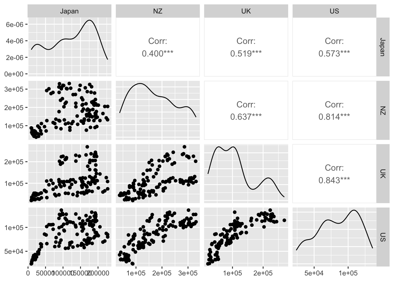
Each point in a plot on the lower diagonal is composed of readings from two time series at the same time point. Note that the plots on the diagonal are density plots, not time plots. A scatterplot with a diagonal pattern suggests that the two time series are very similar. We see something close to this in the UK-US pair, but much less in the JPN-NZ pair.
The upper diagonal entries display Pearson correlations. Unsurprisingly, we can see that the strongest correlation is for the US-UK pair.
3.5 Lag plots
Lag plots are scatter plots in which we plot the values of a time series against those of a time lagged version of itself, i.e. if we denote the time series values by \(x_t\), we plot it against \(x_{t-k}\) for some positive integer \(k\).3 For instance, in Figure 3.6 we display the lag plot for the arrivals to Australia from Japan time series that we’ve been studied so far in this chapter.
aus_arrivals |> filter(Origin == "Japan") %>%
  gg_lag(y = Arrivals, geom = "point") +
  scale_x_continuous(labels = function(x) paste0(x / 1000, "k")) +
  scale_y_continuous(labels = function(x) paste0(x / 1000, "k"))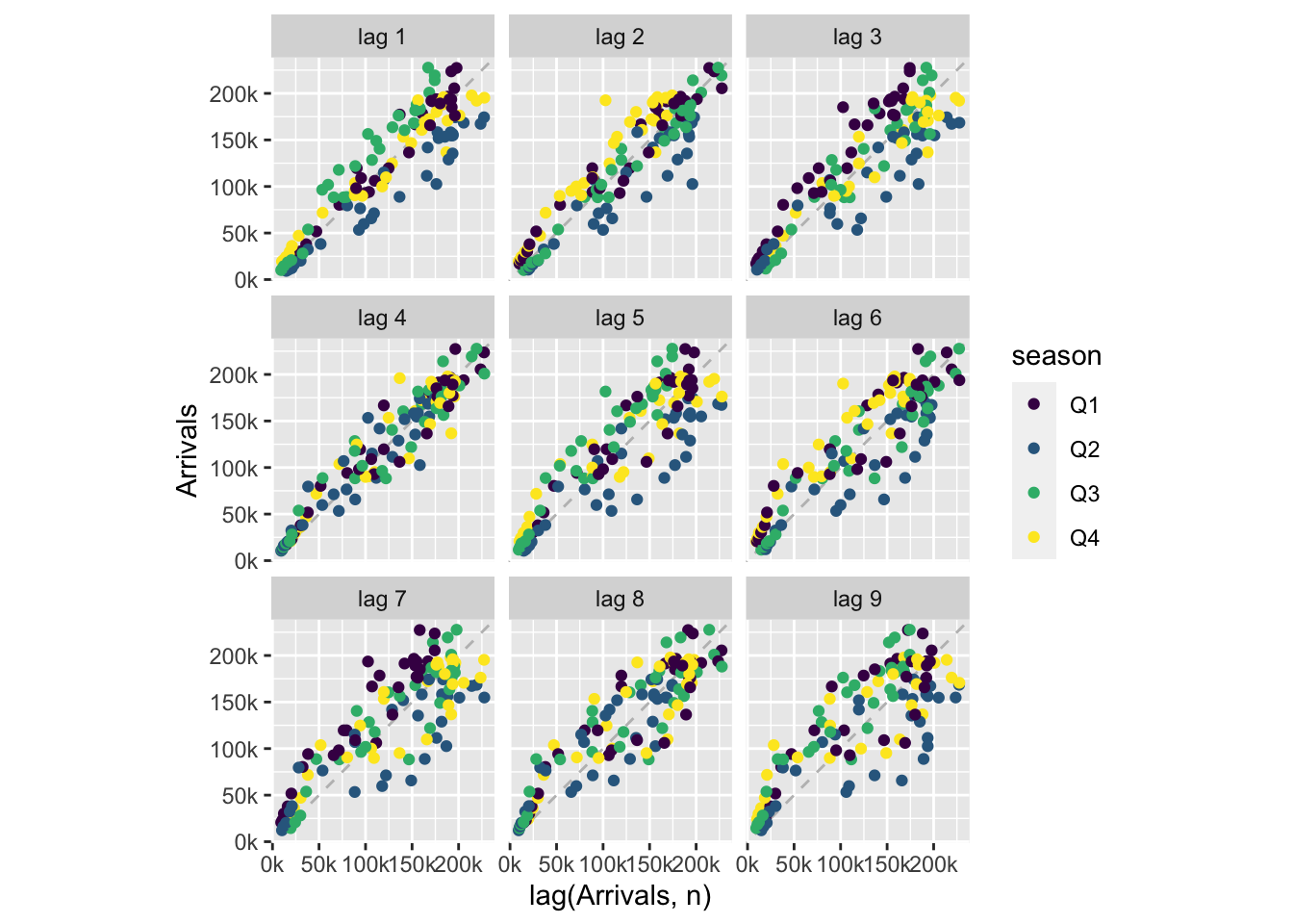
The fact that the scatter plots are close to the diagonal indicates that there is very strong autocorrelation behavior (correlation between the time series and that of its lags). This correlation decays as we take longer and longer lags, but is stronger for lags 4 and 8, indicating yearly seasonality (recall that the time intervals are quarters).
Lag plots are useful for teasing out cyclic patterns. Cyclic patterns occur when the time series values depend on the past values at previous time points (i.e. is autoregressive). This is distinct from trend and seasonality, which are patterns that depend on the time index. Linear autoregressive relationships are efficiently summarized by autocorrelation plots, which will be covered in a latter chapter. Lag plots are less concise than autocorrelation plots, but can demonstrate nonlinear relationships.
gg_lag() has automatically colored coded the different quarters. Can you explain the differences between the patterns observed in different quarters? E.g. for lag 1, why do the Q3 points lie above the diagonal, and why do the Q2 points lie underneath it?