us_change |>
  pivot_longer(c(Consumption, Income), names_to="Series") |>
  autoplot(value) +
  labs(y = "% change")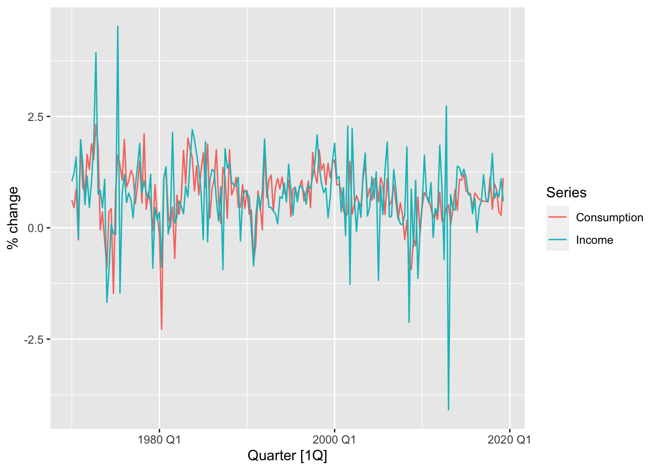
Thus far, we have discussed how to model an individual time series by itself. On the other hand, we usually observe several concurrent time series which could be related to each other. For example, economists interested in understanding the economy of a given country usually have access to multiple economic indicators, such as GDP per capita, unemployment rate, and household wealth (see for instance, the datasets global_economy and hh_budget). These other concurrent time series may be useful in helping to forecast a time series of interest. In addition, the precise causal relationship between different time-varying quantities may also be of interest. For instance, companies are interested in understanding how certain business decisions, such as changing advertisement spend or product pricing, may affect future revenue.
Prediction and causal analysis have long been studied by applying linear regression to sample data from some population. In this chapter, we will learn how to extend linear regression to a time series context.
We begin with a short overview of linear regression. These days, students are likely to first encounter linear regression as a prediction model applied to a given dataset. That is, given a response vector \(\bY = (Y_1,Y_2,\ldots Y_n)^T\) and a covariate matrix \(\bX \in \R^{n \times p}\), the linear regression model is of the form \(\hat f(\bx) = \hat\bbeta^T\bx\), where \[ \hat\bbeta = \arg\min_{\bbeta}\left\|\bY - \bX\bbeta \right\|^2 = (\bX^T\bX)^{-1}\bX^T\bY. \tag{14.1}\]
This prediction algorithm can be derived from a statistical model, which yields additional insight on estimation and predictive uncertainties. There are two types of models, depending on whether we treat the covariates as fixed (called a fixed design), or themselves as random variables (called a random design).1 Assuming a fixed design for now, the response vector is generated according to the formula \[ \by = \bX\bbeta^* + \beps, \tag{14.2}\] where \(\bbeta^*\) is the true regression vector and \(\beps = (\varepsilon_1,\varepsilon_2,\ldots,\varepsilon_n)^T\) is drawn i.i.d. from \(\mathcal{N}(0,\sigma^2)\), for some noise variance parameter \(\sigma^2\). Note that the only randomness is in the response noise vector \(\beps\).
Under these assumptions, one can check that the estimator in Equation 14.1, called the ordinary least squares (OLS) estimator, is also the maximum likelihood estimator. It is an unbiased estimate for \(\bbeta\) and its deviation from the true regression vector satisfies \[ \hat\bbeta - \bbeta^* \sim \mathcal{N}(0, \sigma^2(\bX^T\bX)^{-1}). \] Furthermore, by the Gauss-Markov theorem, the OLS estimator is optimal, in the sense that it has the minimum variance among all unbiased linear estimators of \(\bbeta^*\).
In a random design, the rows of \(\bX\) are assumed to be drawn i.i.d. from a fixed distribution on \(\R^p\) with a covariance matrix \(\bSigma\). Under this assumption, we have the asymptotic behavior: \[ \sqrt{n}(\hat\bbeta - \bbeta^*) \to_d \mathcal{N}(0, \sigma^2\bSigma^{-1}). \]
A linear model is highly interpretable as a predictive (statistical) model. For each \(k=1,2,\ldots,p\), \(\beta_k^*\) is the slope of the prediction surface in the \(k\)-th coordinate direction. In other words, it is the amount by which our prediction increases if we increase the \(k\)-th covariate by 1 unit.
In addition, these coefficient values can sometimes have scientific (also called causal) interpretations. Indeed, one of the earliest uses of linear regression was in randomized experiments. Here, each row in the covariate matrix \(\bX\) corresponds to a particular experimental setting. Equation 14.2 then becomes a causal model, with \(\beta_k^*\) being the effect on the response of increasing the \(k\)-th covariate by 1 unit. Note the subtle difference between this and the earlier interpretation. In a statistical model, \(\beta_k^*\) describes how the prediction would change, given a change in \(X_k\). In a causal model, \(\beta_k^*\) describes how the true value would change if we were to intervene in an experiment to change \(X_k\).
Of course, randomized experiments are not always possible, especially in the social sciences. Economists and sociologists, for instance, usually have to work with non-experimental data coming from census or administative records. Even so, Equation 14.2 can sometimes be justified as a causal model using domain knowledge.
In the setting of multiple time series, we can treat the time series of interest as a response vector \(\bY\) and the remaining time series as columns in a covariate matrix \(\bX\). However, note that because they are measurements of the same time series at different time points, the rows of \(\bX\) are rarely i.i.d.. As such, a random design assumption is unrealistic and we have to use a fixed design interpretation. Focusing on just a single predictor for now, we model \[ Y_t = \alpha + \beta X_t + W_t \tag{14.3}\] for \(t=1,2,\ldots,n\), where \((W_t)\) is a Gaussian white noise process and \((X_t)\) is a fixed (non-random) time series. In the economics literature, \((X_t)\) is sometimes called an exogenous time series, because its dynamics is not modeled.
Let us apply this model to the dataset us_change, which comprises percentage changes in quarterly personal consumption expenditure, personal disposable income, production, savings and the unemployment rate for the US from 1970 to 2016.
us_change |>
pivot_longer(c(Consumption, Income), names_to="Series") |>
autoplot(value) +
labs(y = "% change")
us_change |>
  ggplot(aes(x = Income, y = Consumption)) +
  labs(y = "Consumption (quarterly % change)",
       x = "Income (quarterly % change)") +
  geom_point() +
  geom_smooth(method = "lm", se = FALSE)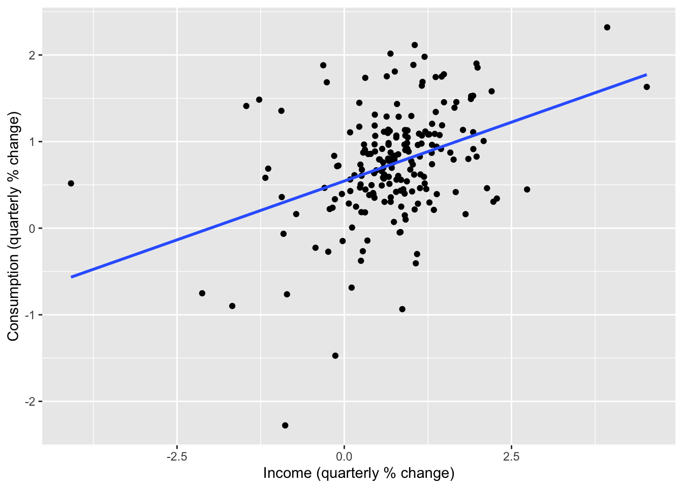
From the time plot and scatter plot shown above, we see that change in income is predictive of change in consumption. This leads us to fit the model Equation 14.3 with these time series as \((X_t)\) and \((Y_t)\) respectively. We do so using the TSLM() function in the fable package.
lr_fit <- us_change |>
  model(TSLM(Consumption ~ Income))
lr_fit |> report()
Series: Consumption
Model: TSLM
Residuals:
Min 1Q Median 3Q Max
-2.58236 -0.27777 0.01862 0.32330 1.42229
Coefficients:
Estimate Std. Error t value Pr(>|t|)
(Intercept) 0.54454 0.05403 10.079 < 2e-16 ***
Income 0.27183 0.04673 5.817 2.4e-08 ***
---
Signif. codes: 0 '***' 0.001 '**' 0.01 '*' 0.05 '.' 0.1 ' ' 1
Residual standard error: 0.5905 on 196 degrees of freedom
Multiple R-squared: 0.1472, Adjusted R-squared: 0.1429
F-statistic: 33.84 on 1 and 196 DF, p-value: 2.4022e-08From the print out, we gather that \(\hat\beta \approx 0.27\) and \(\hat\alpha \approx 0.54\). This can be interpreted as saying that each 1% further increase in income leads to a further 0.27% predicted increase in consumption, and that when income does not change, the predicted increase in consumption is 0.54%.
We now check the goodness of fit of the model via a residual analysis.
lr_fit |> gg_tsresiduals()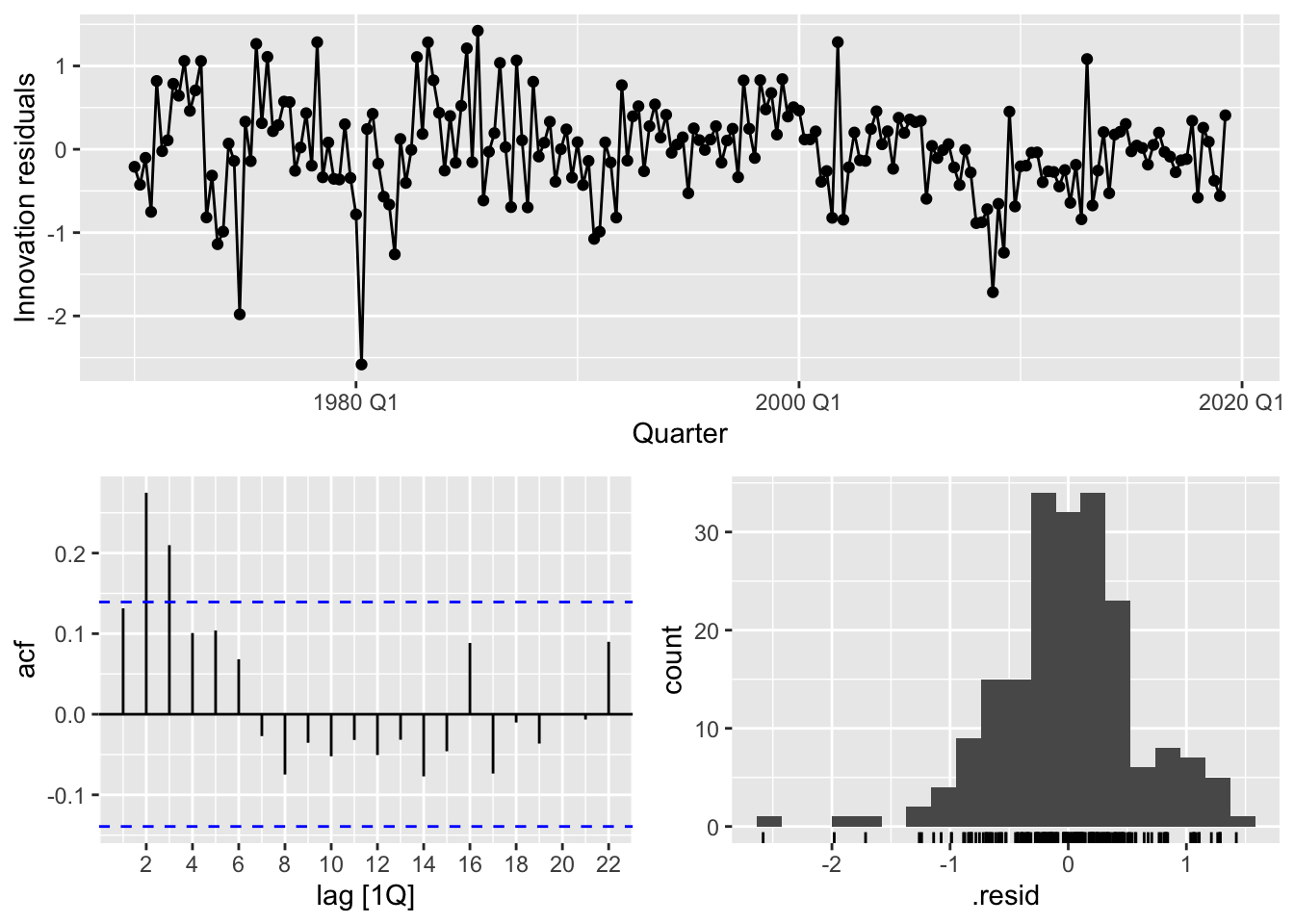
These plots provide evidence that the residuals of the model are not white noise, which violates the modeling assumption in Equation 14.3. This means that we should be suspicious of any conclusions obtained using this model, such as prediction intervals and coefficient interpretations.
Given multiple time fixed time series \((X_{t1}),(X_{t2}),\ldots,(X_{tk})\), we can define the multiple linear regression model \[ Y_t = \alpha + \beta_1 X_{t1} + \cdots \beta_k X_{tk} + W_t \] for \(t = 1,2,\ldots,n\).
Since us_change contains other time series, we can try regressing the change in consumption with multiple predictors. We first make a pairs plot (pairwise scatter plot) to inspect the degree of pairwise marginal correlations between change in consumption and the predictors.
us_change |>
  GGally::ggpairs(columns = 2:6)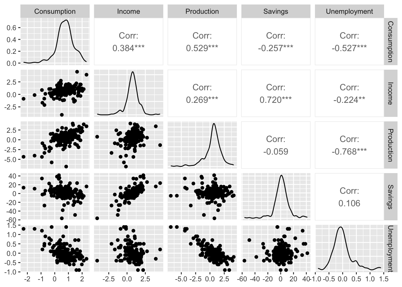
It seems that change in consumption is positively correlated with change in income and change in production, and negatively correlated with change in savings and change in unemployment. Let us now fit the multiple linear regression model.
mlr_fit <- us_change |>
  model(TSLM(Consumption ~ Income + Production + Savings + Unemployment))
mlr_fit |> report()
Series: Consumption
Model: TSLM
Residuals:
Min 1Q Median 3Q Max
-0.90555 -0.15821 -0.03608 0.13618 1.15471
Coefficients:
Estimate Std. Error t value Pr(>|t|)
(Intercept) 0.253105 0.034470 7.343 5.71e-12 ***
Income 0.740583 0.040115 18.461 < 2e-16 ***
Production 0.047173 0.023142 2.038 0.0429 *
Savings -0.052890 0.002924 -18.088 < 2e-16 ***
Unemployment -0.174685 0.095511 -1.829 0.0689 .
---
Signif. codes: 0 '***' 0.001 '**' 0.01 '*' 0.05 '.' 0.1 ' ' 1
Residual standard error: 0.3102 on 193 degrees of freedom
Multiple R-squared: 0.7683, Adjusted R-squared: 0.7635
F-statistic: 160 on 4 and 193 DF, p-value: < 2.22e-16The resulting model is \[ \begin{split} \Delta\text{Consumption}_t & = 0.74\Delta\text{Income}_t + 0.05\Delta\text{Production}_t - 0.05\Delta\text{Savings}_t \\ & \quad - 0.17\Delta\text{Unemployment}_t + 0.25 + W_t. \end{split} \tag{14.4}\]
Notice that the regression coefficient of change of income in Equation 14.4 is different from that of the same predictor in the simple linear regression earlier. Mathematically, this can be explained as the effect of correlations between the predictors. If we believe that Equation 14.4 is the true statistical model, then the difference between the two coefficients is called omitted variable bias. That is, by omitting the other predictors previously, we have biased our estimate of the effect of change of income on change in consumption.
As usual, we check the goodness of fit of this model via a residual analysis.
mlr_fit |> gg_tsresiduals()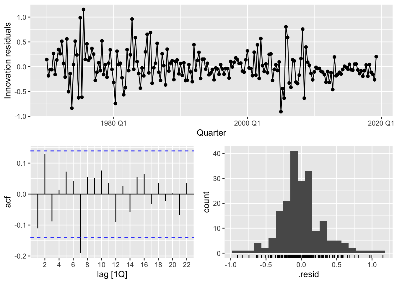
Compared to the simple linear regression model, it seems that the multiple linear regression model in Equation 14.4 has a better fit, which, at face value, suggests that we can trust its conclusions more. Nonetheless, one should still be wary. First, there is a risk that our model has overfit to the observed data and may not remain a good fit at future time points. This can checked via some form of cross-validation. Second, even if the model does not overfit, the phenomenon being modeled may not be stationary, and there is no a priori guarantee that its future behavior will resemble the past. For instance, the relationships between the economic variables in us_change exist under the current economic framework of the country, and may change as a consequence as economics, politics, and technology evolve.
A further issue is that using the regression model to forecast the target time series requires knowledge of the future values of the predictors, which are usually unavailable. If we attempt to use the fitted model in mlr_fit to forecast, R will throw an error warning us that the required predictor values cannot be found.
mlr_fit |> forecast(h = 5)Error in `mutate()`:
ℹ In argument: `TSLM(Consumption ~ Income + Production + Savings +
Unemployment) = (function (object, ...) ...`.
Caused by error in `value[[3L]]()`:
! object 'Income' not found
Unable to compute required variables from provided `new_data`.
Does your model require extra variables to produce forecasts?To resolve this, these predictors can themselves be forecasted, or we may choose to use deterministic predictors instead.
We now discuss useful deterministic predictors that can be used in time series regression. These comprise simple functions in the time index \(t\) that describe commonly seen structure in real-world time series.
Trend: We have already described the linear trend model \(Y_t = \beta_0 + \beta_1 t + W_t\). This is a regression model, where \(t\) is used as the sole predictor. We can extend this in two ways to model potentially nonlinear trend. (i) Apply polynomial functions of \(t\), e.g. we can fit the model \(Y_t = \beta_0 + \beta_1 t + \beta_2 t^2 + W_t\) via the code snippet TSLM(Y ~ trend() + I(trend() ** 2)). (ii) Apply piecewise linear functions of \(t\). We can specify where to place the knots (i.e. points of nonlinearity) via TSLM(Y ~ trend(knots = c(k1, k2, ...))), where k1, k2, and so on are datetime objects corresponding to the knot locations.
Seasonal dummy variables: If the time series is seasonal with period \(m\), we can model it as \[
Y_t = \beta_0 + \beta_1 d_{1,t} + \beta_2 d_{2,t} + \cdots + \beta_{m-1}d_{m-1,t} + W_t,
\] where for \(k=1,\ldots,m-1\), \[
d_{k, t} = \begin{cases}
1 & \text{if}~(t - 1)~\text{mod}~m = k - 1 \\
0 & \text{otherwise}.
\end{cases}
\] In other words, it is a dummy for the \(k\)-th season, with \(\beta_0 + \beta_k\) set to be the mean value of \(Y_t\) during this season. \(d_{1,t},\ldots,d_{m-1,t}\) are called seasonal dummies. Note that the last seasonal dummy is not necessary, because \(d_{m,t} = 1 - \sum_{k=1}^{m-1}d_{k,t}\). We can fit this model via the code snippet TSLM(Y ~ season()).
Outlier dummy variables: If certain observations are outliers, such as when there is a public holiday for a daily time series, they may affect the parameters of our fitted model in an undesirable way. To counteract this, we may use a dummy for that time point as a predictor. In fable, we can create a new column that is equal to 1 for that time point and equal to 0 otherwise, and add that as a predictor in TSLM().
There are two obvious problems with the time series regression model Equation 14.4. First, it is not able to model lagged effects of the predictors on the response time series. We have already noted in Chapter 12 that lagged effects is a common feature of time series analysis and is a motivation for the class of MA(\(q\)) models. Second, it does not allow for the possibility that the regression residuals have nonzero autocorrelation. When there is indeed such autocorrelation, naively applying time series regression can lead to issues such as inefficient estimation of the regression coefficients.
These problems are addressed by performing dynamic regression. Given a single predictor time series \((X_t)\), this corresponds to the model \[ Y_t = \beta_0 + \beta_{1,0}X_t + \beta_{1,1}X_{t-1} + \cdots + \beta_{1,r}X_{t-r} + \eta_t, \] where \((\eta_t)\) is drawn from an ARIMA model.
Such a model can be fit by specifying \((X_t)\) and its lags as additional predictor in the ARIMA() function in fable. While the desired lags to be used need to be explicitly specified, the precise ARIMA model to be used can be automatically estimated from data, as is the case with vanilla ARIMA modeling. We demonstrate this by fitting two dynamic regression models using the us_change dataset.
consumption_fit <- us_change |>
  model(dr1 = ARIMA(Consumption ~ Income),
        dr2 = ARIMA(Consumption ~ Income + lag(Income, 1)))
consumption_fit |> select(dr1) |> report()
Series: Consumption
Model: LM w/ ARIMA(1,0,2) errors
Coefficients:
ar1 ma1 ma2 Income intercept
0.7070 -0.6172 0.2066 0.1976 0.5949
s.e. 0.1068 0.1218 0.0741 0.0462 0.0850
sigma^2 estimated as 0.3113: log likelihood=-163.04
AIC=338.07 AICc=338.51 BIC=357.8Above, we report the fitted parameters under the first model, dr1. We see that the fitted model can be written as \[
\Delta\text{Consumption}_t = 0.59 + 0.20\Delta\text{Income}_t + \eta_t
\] \[
\eta_t = 0.71\eta_{t-1} + W_t -0.62W_{t-1} + 0.21 W_{t-2}
\] \[
W_t \sim N(0, 0.31).
\]
Compared to the simple linear regression model earlier, we see that we get a different set of estimates for both the intercept as well as the regression coefficient for \(\Delta\text{Income}_t\) (change in income). We now perform a residual analysis.
consumption_fit |> select(dr1) |> gg_tsresiduals()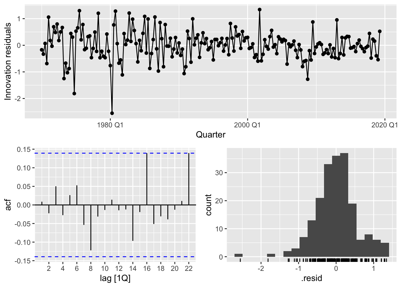
This seems to suggest a better fit. However, there are still some skewness in the residuals, as well as some outlier values, such as in 1980 Q1.
As is the case with vanilla linear regression, dynamic regression can be extended to involve multiple predictor time series.
The parameters of a dynamic regression model can be estimated using maximum likelihood as before. However, one needs to be careful about potential multicollinearity affecting the stability of this estimation process. Specifically, if any of the predictor time series is non-stationary, it can potentially have high correlation with an ARIMA time series, which leads to inefficiency and even unidentifiability when estimating the parameters. As such, it is good practice to take enough differences to ensure that all predictors (and the response) are stationary, before applying dynamic regression.
Likewise, model selection can be done by making use of AIC and AICc. Unlike with ARIMA models, however, the fable package does not automatically select from models with different choices of predictors or with different numbers of lags of these predictors. One has to do this manually by simultaneously fitting multiple candidate models and comparing their reported AICc values.
Let us illustrate this again with the us_change dataset. In the following, we fit a few models to predict change in consumption and compare their relative AICc values. Note that all time series in the dataset already appear to be stationary, so no further differencing is required.
consumption_fit <- us_change |>
  model(dr1 = ARIMA(Consumption ~ Income + lag(Income, 1)),
        dr2 = ARIMA(Consumption ~ Income + lag(Income, 1) + Production +
                    lag(Production, 1)),
        dr3 = ARIMA(Consumption ~ Income + lag(Income, 1) + Production +
                    lag(Production, 1) + Unemployment + lag(Unemployment, 1)),
        dr4 = ARIMA(Consumption ~ Income + lag(Income, 1) + Production +
                    lag(Production, 1) + Unemployment + lag(Unemployment, 1) +
                    Savings + lag(Savings, 1)),
        dr5 = ARIMA(Consumption ~ Income + lag(Income, 1) + Production +
                    lag(Production, 1) + Unemployment + lag(Unemployment, 1) +
                    Savings + lag(Savings, 1) + lag(Income, 2) + lag(Production, 2) +
                    lag(Unemployment, 2) + lag(Savings, 2)))
consumption_fit |> glance()
# A tibble: 5 × 8
.model sigma2 log_lik AIC AICc BIC ar_roots ma_roots
<chr> <dbl> <dbl> <dbl> <dbl> <dbl> <list> <list>
1 dr1 0.291 -154. 327. 328. 356. <cpl [11]> <cpl [0]>
2 dr2 0.241 -137. 287. 287. 307. <cpl [0]> <cpl [0]>
3 dr3 0.228 -131. 277. 278. 304. <cpl [0]> <cpl [0]>
4 dr4 0.0966 -43.4 117. 119. 166. <cpl [12]> <cpl [0]>
5 dr5 0.0915 -36.3 111. 115. 173. <cpl [12]> <cpl [0]>Surprisingly, the model that has the smallest AICc value is the most complicated model, which includes the current value and the first two lags of all the possible predictor time series. A residual analysis seems to suggest that the model is a good fit.
consumption_fit |> select(dr5) |> gg_tsresiduals()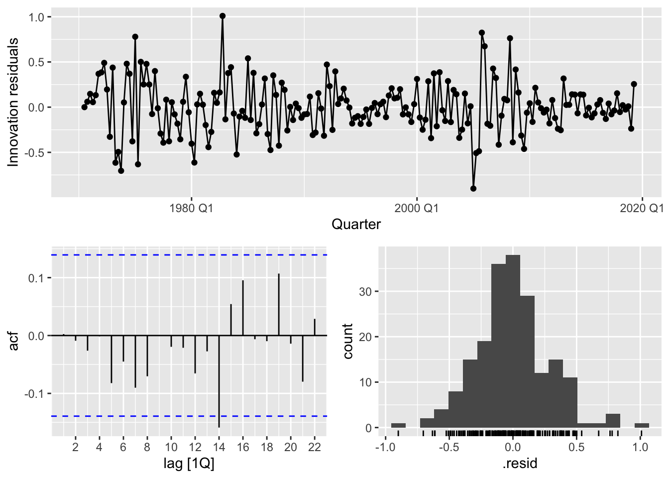
Instead of following a two-stage process whereby we first forecast the predictor time series and then use their forecasted values to forecast the regression target, one may model all time series simultaneously via a vector autoregression (VAR) model. In this case, we concatenate all time series of interest into a vector \(\bX_t = (X_{1t}, X_{2t},\ldots,X_{kt})\). A vector autoregression model of order \(p\), denoted VAR(\(p\)), has the form
\[ \bX_t = \balpha + \bPhi_1 \bX_{t-1} + \bPhi_2 \bX_{t-2} + \cdots + \bPhi_p\bX_{t-p} + \bW_t, \] where \(\bPhi_1,\bPhi_2,\ldots,\bPhi_p\) are \(k \times k\) coefficient matrices, and \(\bW_t \sim N(0, \bSigma)\) for some covariance matrix \(\bSigma\), with \(\bW_s\) and \(\bW_t\) independent whenever \(s \neq t\).
Modeling with VAR helps to streamline forecasting because one can simply perform recursive forecasting. VAR models are similar to AR(\(p\)) models in other ways, with most concepts for AR(\(p\)) models having natural analogues. For example, stationarity of a VAR model has to do with the unit roots of the VAR polynomial. Furthermore, VAR models can be extended to vector ARMA models to gain even more flexibility.
The downside of using a VAR model is that it often requires a large number of parameters. For example, if we had modeled each of the \(k\) time series in \((\bX_t)\) individually as an AR(\(p\)) model, we would need to estimate \(kp\) parameters (not including the constant coefficient and noise variances). Modeling them using a VAR(\(p\)) model requires \(k^2p\) parameters instead. Having too many parameters makes estimation difficult as it inflates the sampling variance of any reasonable estimator and makes it more likely for any fitted model to be overfit. Therefore, a common practice is to set some (or even most) entries of the coefficient matrices to be zero. Deciding which entries are allowed to be nonzero is part of the problem of model selection for VAR(\(p\)) models, and can be done by comparing AICc values as before.
In the fable package, a VAR model can be fit using the VAR() function. We illustrate how to do this using us_change dataset as before. In the following code snippet, we model the two time series measuring change in consumption and change in income jointly. Note how they are concatenated symbolically using the vars() function.
consumption_fit <- us_change |>
  model(VAR(vars(Consumption, Income)))
consumption_fit
# A mable: 1 x 1
`VAR(vars(Consumption, Income))`
<model>
1 <VAR(5) w/ mean>Because we did not indicate what order \(p\) to select, this was automatically determined using AICc, and selected to be \(p=5\). Displaying the fitted coefficients below, we observe that all coefficients for the VAR(\(5\)) model were estimated. It seems that the package does not have functionality to fix certain parameters at zero.
consumption_fit |>
  tidy() |> select(-.model) |> print(n = 22)
# A tibble: 22 × 6
term .response estimate std.error statistic p.value
<chr> <chr> <dbl> <dbl> <dbl> <dbl>
1 lag(Consumption,1) Consumption 0.186 0.0771 2.42 0.0166
2 lag(Income,1) Consumption 0.112 0.0535 2.09 0.0379
3 lag(Consumption,2) Consumption 0.166 0.0792 2.09 0.0378
4 lag(Income,2) Consumption -0.0117 0.0563 -0.207 0.836
5 lag(Consumption,3) Consumption 0.302 0.0789 3.82 0.000182
6 lag(Income,3) Consumption -0.0315 0.0551 -0.571 0.569
7 lag(Consumption,4) Consumption -0.0291 0.0818 -0.356 0.722
8 lag(Income,4) Consumption -0.0754 0.0552 -1.37 0.173
9 lag(Consumption,5) Consumption -0.0492 0.0781 -0.630 0.529
10 lag(Income,5) Consumption -0.0433 0.0529 -0.819 0.414
11 constant Consumption 0.350 0.0870 4.02 0.0000852
12 lag(Consumption,1) Income 0.402 0.109 3.70 0.000288
13 lag(Income,1) Income -0.299 0.0754 -3.97 0.000104
14 lag(Consumption,2) Income 0.102 0.112 0.917 0.361
15 lag(Income,2) Income -0.0449 0.0793 -0.566 0.572
16 lag(Consumption,3) Income 0.469 0.111 4.21 0.0000397
17 lag(Income,3) Income -0.148 0.0777 -1.91 0.0578
18 lag(Consumption,4) Income 0.259 0.115 2.24 0.0262
19 lag(Income,4) Income -0.252 0.0778 -3.24 0.00144
20 lag(Consumption,5) Income -0.126 0.110 -1.15 0.253
21 lag(Income,5) Income -0.197 0.0746 -2.64 0.00891
22 constant Income 0.575 0.123 4.69 0.00000543To inspect the goodness of fit, we plot the ACF of the model residuals for both change in consumption and change in income. Since gg_tsresiduals() no longer works for a multivariate model, we use the following code snippet. The ACF plots seem to suggest that the model is a relatively good fit, but one should also be sure to check the time plot and density plot for further verification.
consumption_fit |>
  augment() |>
  ACF(.innov) |>
  autoplot()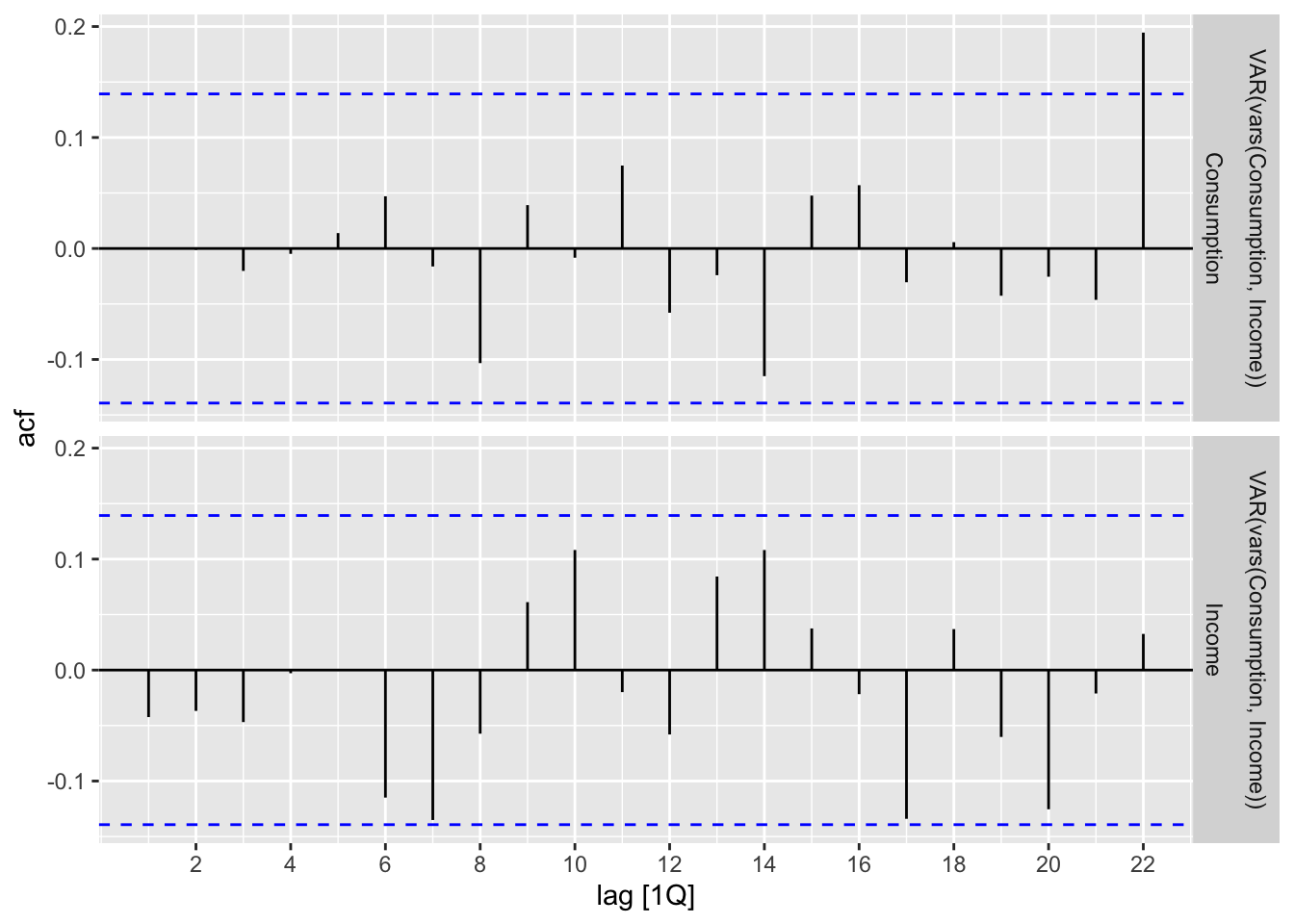
Finally, we can use the fitted model to forecast.
consumption_fit |>
  forecast(h = 20) |>
  autoplot(us_change)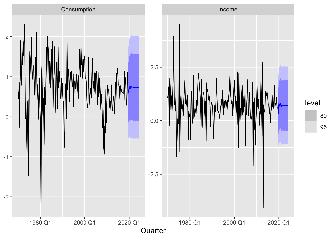
In this section, we explain how to combine ideas from regression and spectral analysis to address a critical limitation of seasonal ARIMA models. While seasonal ARIMA models have the ability to model seasonality, it experiences difficulty in working with long seasonal periods. This is because when the seasonal period is long, such as when there is yearly seasonality for an hourly time series, there may not be enough observations within the same seasonal period (i.e. 9am on April 10) to form reliable forecasts. Using either the Holt-Winters method or seasonal dummies in a time series regression also runs into similar issues: The number of coefficients to be estimated is at least the length of the seasonal period.
To address this, we can include Fourier (i.e. sinusoidal) functions as predictors. Recall that these are sine and cosine functions in the time index \(t\) of various frequencies, and that they form a basis for \(\R^n\). By only using the lower frequency terms, we can fit slow-varying seasonal structures with only a small number of parameters, thereby preserving model simplicity. Making use of these predictors and combining with ARIMA errors is called dynamic harmonic regression.
Some authors refer to what we just described above as “dynamic harmonic regression with ARIMA errors” (DHR-ARIMA), and reserves the term “dynamic harmonic regression” to refer to regression against Fourier predictors with white noise errors.
Another advantage of dynamic harmonic regression is that we can model non-integer seasonalities, e.g. weekly seasonality if we have measurements only once every two days.
To illustrate the use of this new tool, we apply it to the diabetes dataset, which we recall is a monthly time series with yearly seasonality.
diabetes <- readRDS("_data/cleaned/diabetes.rds")
diabetes_dhr_fit <- diabetes |>
  model(ARIMA(log(TotalC) ~ fourier(K = 6)))
diabetes_dhr_fit
# A mable: 1 x 1
`ARIMA(log(TotalC) ~ fourier(K = 6))`
<model>
1 <LM w/ ARIMA(1,1,1)(0,0,1)[12] errors>We specify using Fourier predictors via the syntax fourier(K = 6), where K is used to specify using the frequencies \(1/T, 2/T, \ldots, 6/T\). \(T\) is used to denote the seasonal period, which is equal to 12 in this example. Since we did not specify the order of the ARIMA model, it is automatically estimated from data. We view the values of the fitted coefficients below.
diabetes_dhr_fit |> tidy() |> select(-.model)# A tibble: 15 × 5
term estimate std.error statistic p.value
<chr> <dbl> <dbl> <dbl> <dbl>
1 ar1 -0.167 0.0968 -1.73 8.57e- 2
2 ma1 -0.739 0.0766 -9.65 2.18e-18
3 sma1 0.268 0.0878 3.06 2.55e- 3
4 fourier(K = 6)C1_12 0.0597 0.00602 9.91 4.03e-19
5 fourier(K = 6)S1_12 -0.115 0.00607 -18.9 1.26e-46
6 fourier(K = 6)C2_12 0.0628 0.00570 11.0 1.99e-22
7 fourier(K = 6)S2_12 -0.0737 0.00572 -12.9 3.66e-28
8 fourier(K = 6)C3_12 0.0473 0.00602 7.87 2.10e-13
9 fourier(K = 6)S3_12 -0.0564 0.00602 -9.37 1.40e-17
10 fourier(K = 6)C4_12 0.0532 0.00653 8.16 3.55e-14
11 fourier(K = 6)S4_12 -0.0284 0.00653 -4.35 2.18e- 5
12 fourier(K = 6)C5_12 0.0392 0.00702 5.59 7.35e- 8
13 fourier(K = 6)S5_12 -0.0370 0.00703 -5.26 3.57e- 7
14 fourier(K = 6)C6_12 0.0295 0.00511 5.78 2.83e- 8
15 intercept 0.00969 0.00112 8.66 1.43e-15Observe that 12 Fourier functions were used in the regression, comprising sine and cosine functions with the frequencies described earlier, i.e. \(\sin(2\pi t/ 12), \cos(2\pi t/12), \sin(2\pi t / 6), \cdots\). The most dominant frequency is \(\omega = 1/12\), which agrees with what one would observe from a periodogram plot. We now visualize the forecasts as follows:
diabetes_dhr_fit |>
  forecast(h = 24) |>
  autoplot(diabetes)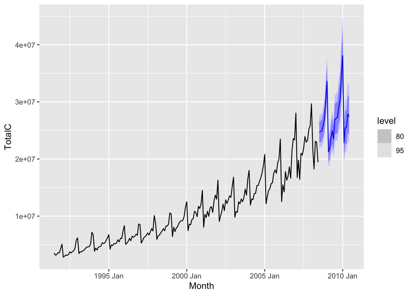
Next, we consider the vic_elec, which records energy consumption in Victoria, Australia. Recall from Chapter 5 that this is a half-hourly time series that displays multiple seasonality, with daily, weekly, and yearly periods. Such complex seasonality is especially hard to model using either ARIMA or ETS models. We can tailor our model to this complex seasonality via using three sets of Fourier terms, corresponding to the different seasonal periods. We also specify the number of Fourier terms to be used for each seasonal period.
elec_dhr_fit <- vic_elec |>
  model(dhr = ARIMA(Demand ~ fourier(period = "day", K = 10) +
                    fourier(period = "week", K = 5) +
                    fourier(period = "year", K = 3)))
Although simple, dynamic harmonic regression is a powerful forecasting method that, with appropriate feature engineering, has been observed to outperform even state-of-the-art deep learning methods on many datasets.
A major goal of any scientific discipline is understanding causality. This includes causal discovery, which means identifying potential factors causing a given natural phenomenon, such as lung cancer, tornado formation, or economic recession, as well as causal estimation, which means estimating the degree and manner in which each of these factors affects the quantity of interest. Causal estimation can sometimes be performed using randomized experiments, as discussed earlier in this chapter. On the other hand, randomized experiments are not always economically, ethically, or practically feasible. For instance, it is impossible to experiment on countries’ economic policies in order to understand what might cause an economic recession. Researchers hence often have to make use of observational data.
However, naively drawing causal conclusions from observational data can be extremely misleading, as even strong correlations that exist may be a result of various types of confounding, selection bias, or sheer randomness, rather than of a causal relationship. This is especially true for non-stationary time series data, given the small sample size for many such datasets and the limited number of possible patterns. Such relationships are called spurious correlations. This website curates a collection of often humorous spurious correlations.
In order to draw reliable causal conclusions, researchers have sought to define causality quantitatively via various frameworks. One such framework is Granger causality, which makes use of time series data. The idea is as follows. Given two time series \((X_t)\) and \((Y_t)\), we say that \((X_t)\) Granger causes \((Y_t)\) if the dynamic regression model of \((Y_t)\) given \((X_t)\) is a better fit than a univariate AR model of \((Y_t)\). The intuition is that if past values of \((X_t)\) are predictive of future values of \((Y_t)\), even after adjusting for previous values of \((Y_t)\), then there is some evidence that \((X_t)\) has a causal effect on \((Y_t)\).
More precisely, we formulate the following pair of null and alternate hypotheses: \[ H_0: \quad Y_t = \sum_{i=1}^p \phi_i Y_{t-i} + \phi_0 + W_t \]
\[ H_1: \quad Y_t = \sum_{i=1}^p \phi_i Y_{t-i} + \sum_{i=1}^p \beta_i X_{t-i} + \phi_0 + W_t \tag{14.5}\] where \((W_t) \sim WN(0,\sigma^2)\), and \(p\) is estimated via AICc. To check whether Equation 14.5 is a better fit, one uses the F-test. The test statistic is \[ F = \frac{(RSS_{0}- RSS_{1})/p}{RSS_1/(n-2p-1)}, \] where \(RSS_0\) and \(RSS_1\) denote the sum of squared residuals under \(H_0\) and \(H_1\) respectively. Under \(H_0\), \(F\) has the \(F\)-distribution with \(p\) and \(n-2p-1\) degress of freedom.
Let us try to see if change in income Granger causes change in consumption, using the us_change dataset. To start, we first fit an AR model for the change in consumption time series.
h0_fit <- us_change |>
  model(AR(Consumption))
h0_fit
# A mable: 1 x 1
`AR(Consumption)`
<model>
1 <AR(5) w/ mean>We see that a model of order \(p=5\) was selected using AICc. We then fit a VAR model of order \(p=5\) to both change in consumption and change in income, and extract the sum of squared residuals of both models.
h1_fit <- us_change |>
  model(VAR(vars(Consumption, Income) ~ AR(5)))
h0_resid <- h0_fit |>
  augment() |>
  pull(.innov)
h1_resid <- h1_fit |>
  augment() |>
  filter(.response == "Consumption") |>
  pull(.innov)
h0_rss <- h0_resid ** 2 |>
  mean(na.rm = TRUE)
h1_rss <- h1_resid ** 2 |>
  mean(na.rm = TRUE)
To compute the p-value, we use the CDF of the relevant F distribution.
df1 <- 5
df2 <- nrow(us_change) - 11
F <- ((h0_rss - h1_rss) / df1) / (h1_rss / df2)
p_val <- 1 - pf(F, df1, df2)
p_val
[1] 0.1386631The p-value is relatively large, so we do not have enough evidence to conclude that change in income Granger causes change in consumption.
Granger causality has been widely applied in economics as well as neuroscience. However, there is still controversy about whether Granger causality really implies causality in a mechanistic sense, since it is still based on some form of statistical correlation rather than experimental interventions.
This terminology seems to have come from the literature on design of experiments.↩︎