9 Spectral Analysis
9.1 Introduction to Fourier analysis
In the 19th century, mathematician and physicist Joseph Fourier discovered that all periodic functions can be written as a sum of sine and cosine waves of various frequencies. Analyzing functions in terms of its frequencies, now called Fourier analysis, provided an important tool for solving differential equations, which had numerous immediate applications for the study of physics and engineering. This idea also turns out to be very fruitful in time series analysis and is the starting point for the approach called spectral analysis.
9.2 Fourier coefficients
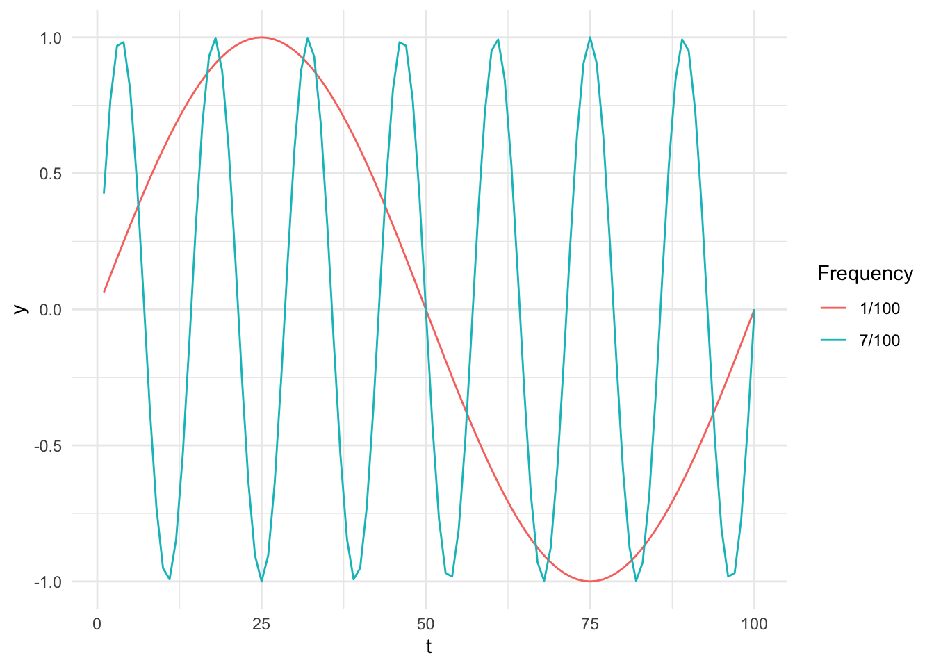
Suppose we have a time series \((y_t)_{t=1}^n\), and assume for now that \(n\) is even. For any \(j=1,2,\ldots, n/2\), consider the sequences \((s_{jt})_{t=1}^n\) and \((c_{jt})_{t=1}^n\), where \[ s_{jt} = \sin(2\pi t j/n), \quad\quad c_{jt} = \cos(2\pi t j/n). \] These can be taught of as periodic functions in the time index \(t\), with \(j/n\) measuring the frequency of the function. For \(n=100\), the sequences \((s_{jt})\) for \(j=1/100\) and \(j= 7/100\) are plotted below.
Removing \((s_{n/2, t})\), which is identically zero1, and adding the constant sequence, one can show that, after normalizing by \(\sqrt{2/n}\), these sequences form an orthonormal basis for \(\R^n\), called the Fourier basis. In other words, we have
Proposition 9.1. (Orthogonality relations) The sequences \((s_{jt})_{t=1}^n\) and \((c_{jt})_{t=1}^n\) for \(j=1,2,\ldots, n/2\) satisfy \[ \frac{2}{n}\sum_{t=1}^n s_{jt}s_{kt} = \begin{cases} 1 & \text{if}~j = k \\ 0 & \text{otherwise}, \end{cases} \] \[ \frac{2}{n}\sum_{t=1}^n c_{jt}c_{kt} = \begin{cases} 1 & \text{if}~j = k \\ 0 & \text{otherwise}, \end{cases} \] \[ \frac{2}{n}\sum_{t=1}^n s_{jt}c_{kt} = 0. \]
The Fourier coefficients \(a_j\) and \(b_j\) are the regression coefficients when regressing the time series \((y_t)\) onto this basis. Because of the orthogonality relations, we have the convenient formulas: \[ a_j = \frac{2}{n} \sum_{t=1}^n y_t c_{jt}, \quad\quad b_j = \frac{2}{n} \sum_{t=1}^n x_t s_{jt}. \tag{9.1}\]
To prove this, define the \(n \times n\) matrix \[ \bZ = \begin{bmatrix} \frac{1}{\sqrt{2}} & \cos\left( 2\pi \frac{1}{n} \cdot 1 \right) & \sin\left( 2\pi \frac{1}{n} \cdot 1 \right) & \cos\left( 2\pi \frac{2}{n} \cdot 1 \right) & \dots & \cos\left( 2\pi \frac{n/2}{n} \cdot 1 \right) \\ \frac{1}{\sqrt{2}} & \cos\left( 2\pi \frac{1}{n} \cdot 2 \right) & \sin\left( 2\pi \frac{1}{n} \cdot 2 \right) & \cos\left( 2\pi \frac{2}{n} \cdot 2 \right) & \dots & \cos\left( 2\pi \frac{n/2}{n} \cdot 2 \right) \\ \vdots & \vdots & \vdots & \vdots & \ddots & \vdots \\ \frac{1}{\sqrt{2}} & \cos\left( 2\pi \frac{1}{n} \cdot n \right) & \sin\left( 2\pi \frac{1}{n} \cdot n \right) & \cos\left( 2\pi \frac{2}{n} \cdot n \right) & \dots & \cos\left( 2\pi \frac{n/2}{n} \cdot n \right) \end{bmatrix}. \] The regression coefficients of \(\by = (y_t)\) on the Fourier basis are given by the formula \[ (\bZ^T\bZ)^{-1}\bZ^T\by. \] However, it is easy to check that the orthogonality relations imply \(\bZ^T\bZ = \frac{n}{2}\bI\), where \(\bI\) is the identity matrix. This means that each entry of \((\bZ^T\bZ)^{-1}\bZ^T\by\) is of the form Equation 9.1.
When \(n\) is odd, we simply enumerate over \(j=1,2,\ldots,(n-1)/2\) (and add the constant sequence as before).
The Fourier coefficients of \((y_t)\) tell us to what extent each frequency is represented in the time series. Hence, they can be interpreted as summary statistics for time series. Beyond that, because the Fourier basis is a basis, the mapping from \((y_t)\) to its Fourier coefficients (this map is called the Fourier transform) is invertible. Indeed, if we set \(\ba \coloneqq (\bZ^T\bZ)^{-1}\bZ^T\by\), we have \[ \bZ\hat\ba = \bZ(\bZ^T\bZ)^{-1}\bZ^T\by = \by. \] Written in terms of \((s_{jt})\) and \((c_{jt})\), we have \[ y_t = \bar{y} + \sum_{j=1}^{n/2} \left( a_j c_{jt} + b_j s_{jt}\right). \]
9.3 Periodogram
Using the trigonometric identity \[ \cos(u+v) = \cos(u)\cos(v) - \sin(u)\sin(v), \] we see that \[ a_jc_{jt} + b_j s_{jt} = \sqrt{a_j^2 + b_j^2} \cos(2\pi t j/n + \phi), \] where \(\phi = \arctan(-b_j/a_j)\). This is a single sine curve with amplitude \(\sqrt{a_j^2 + b_j^2}\) and phase \(\phi\).
In time series analysis, we often are more interested in the amplitude of the frequency and are not particular interested in the phase. This leads to the definition of the periodogram \(P\), which is defined as the function \[ P(j/n) \coloneqq \frac{n^2}{4}\left(a_j^2 + b_j^2\right), \] for \(j=1,2,\ldots,n/2\). Note that \(j/n\) is equal to the frequency, its reciprocal \(n/j\) is equal to its period (the length of the repeating unit), and \(P(j/n)\) is the squared amplitude (also known as intensity) of that frequency. The factor of \(n^2/4\) is unimportant since we are only interested in relative values. Its presence will be explained later.
To illustrate the use of the periodogram, we will investigate two examples.
9.3.1 Star magnitude
We make use of the star dataset provided by the astsa package (Shumway and Stoffer (2000)). This dataset comprises observations of the mangitude of a star taken at midnight for 600 consecutive days. The time plot and the periodogram (truncated at 0.08 for better resolution) are shown below.
star |>
    as_tsibble() |>
    rename(Day = index, Value = value) |>
    autoplot() + labs(y = "Star magnitude")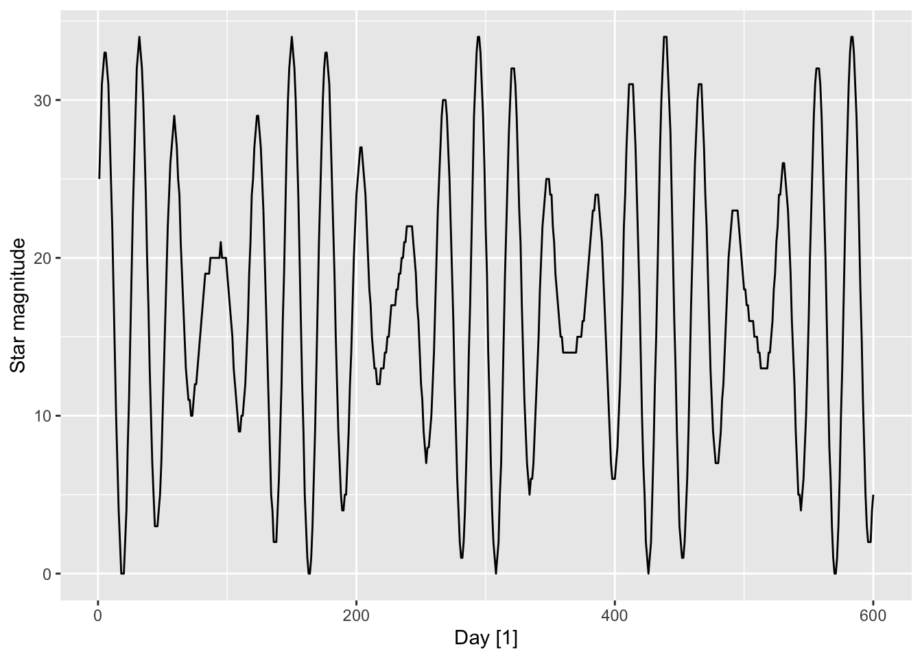
star |>
    periodogram(max_freq = 0.08)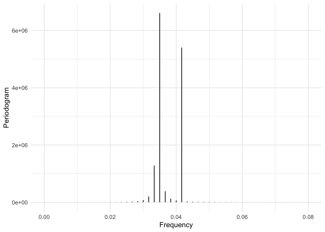
To interpret the periodogram, we see that there are two peaks, occuring at frequencies roughly 0.04167 and 0.35. These corresponds to periods of roughly \(24 \approx 1/0.04167\) days and \(29 \approx 1/0.35\) days respectively. The strength of these peaks is suggestive of the star magnitude being mostly determined by stable astrophysical phenomena of a periodic nature.
9.3.2 Lynx furs
We plot the periodogram for the Hudson Bay Company trading records for lynx furs, contained in the pelt dataset.
pelt |>
    autoplot(Lynx)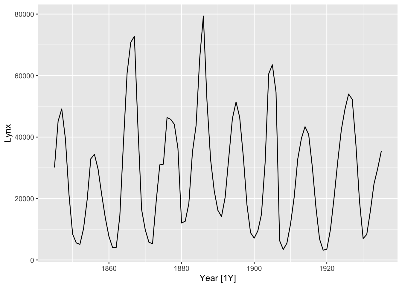
pelt$Lynx |>
    periodogram(max_freq = 0.5)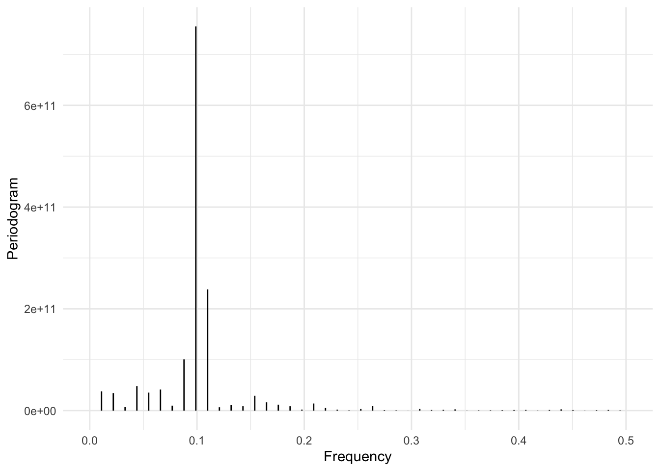
We see that there is a peak at frequency = 0.1, which corresponds to In comparison to a period of \(10 = 1/0.1\) years. This agrees with the ACF plot for the same time series (Figure 8.7). The more diffuse nature of this peak suggests that the periodic pattern is not as stable as in the previous example.
9.3.3 US retail employment
For the last example, we will work US employment data contained in us_employment, focusing on employment numbers in the retail sector.
us_retail_employment <- us_employment |>
  filter(year(Month) >= 1990, Title == "Retail Trade") |>
  select(-Series_ID, -Title)
We perform an STL decomposition and then plot the periodogram of the detrended time series.
us_retail_employment |>
    model(STL(Employed)) |>
    components() |>
    autoplot()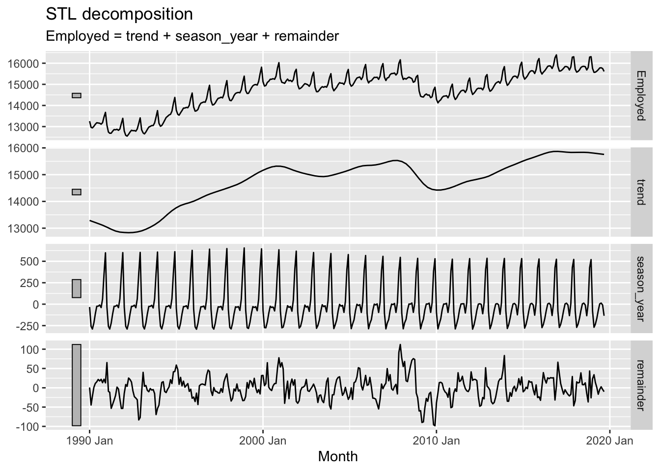
us_retail_employment |>
    model(STL(Employed)) |>
    components() |>
    mutate(trend_adjust = Employed - trend) |>
    pluck("trend_adjust") |>
    periodogram()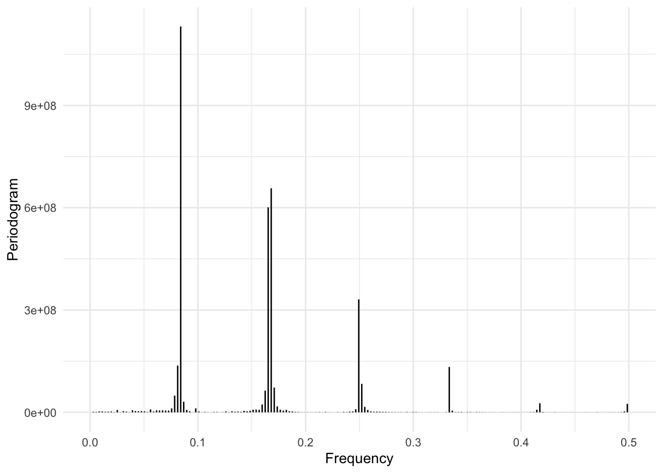
There are peaks approximately at frequencies 0.08, 0.16, 0.25 and 0.33. Bearing in mind that this is a monthly time series, these correspond to periods of 12 months, 6 months, 4 months, and 3 months respectively. These are all divisors of 12, which means that the sinusoidal functions corresponding to these frequencies all contribute to building the yearly (12 month) seasonal unit. The relative height of the peaks suggests that the yearly seasonality is the strongest.
Note that if we do not detrend the time series before generating the periodogram, we get a very different and more ambiguous result, since frequencies of all orders are required to generate the non-periodic trend component.
9.4 Applications of spectral analysis
Spectral analysis is a rich area that has many uses cases. As seen from the above discussion, it allows us to identify cyclic patterns more reliably than with seasonal or ACF plots. Seasonal plots require estimation of the relevant seasonal period, which is then usually constrained to a few rigid choices (e.g. yearly, monthly, weekly, hourly). ACF plots usually mask all but the most dominant frequency. In comparison, the periodogram reveals a finer resolution of what frequencies are present and allows us to compare their relative strengths.
When the periodogram is sparse, i.e. when only a few frequencies are significant, the nonzero Fourier coefficients provide useful features that can be used for time series classification or clustering. By selecting certain frequencies and zeroing out the others, we also obtain transformations that can isolate long-term trends or rapid fluctuations, thereby supplementing the tools we already have for time series decomposition.
Spectral analysis is also useful for forecasting. One of the most broadly used model is DHR-ARIMA, which stands for dynamic harmonic regression with ARIMA errors. This combines ARIMA modeling (Chapter 13) with regression onto sinusoidal terms of certain frequencies. We will learn more about this in a later chapter.
9.5 *Computing periodograms in R using the FFT
Computing Fourier coefficients via the formulas Equation 9.1 can be computationally expensive when the length of the time series \(n\) is large. Indeed, the running time is \(O(n^2)\). One of the biggest engineering breakthroughs in the 20th century was the discovery of an algorithm, called the Fast Fourier transform (FFT), that is able to compute the Fourier transform in \(O(n\log n)\) time.
The FFT is defined in terms of complex exponentials, making use of Euler’s identity \[ e^{i\theta} = \cos(\theta) + i\sin(\theta), \] where \(i\) refers to imaginary unit (satisfying \(i^2 = -1\)). The (complex) Fourier coefficients of \((y_t)\) are defined as \[ \hat y_j \coloneqq \sum_{t=1}^n y_t e^{-2\pi i tj/n}. \tag{9.2}\] Using Euler’s identity, the coefficients \(a_j\) and \(b_j\) (defined in Equation 9.1) can be computed as the real and imaginary parts of \(\hat y_j\) (after normalization). In turn the periodogram can be computed as \[ \begin{split} P(j/n) & = \frac{n^2}{4}\left(a_j^2 + b_j^2\right) \\ & = \frac{n^2}{4}\left(\text{Re}(\frac{2}{n}\hat y_j)^2 + \text{Im}(\frac{2}{n}\hat y_j)^2\right) \\ & = \text{Re}(\hat y_j)^2 + \text{Im}(\hat y_j)^2 \\ & = \left|\hat y_j \right|^2. \end{split} \]
We can express Equation 9.2 concisely as \[ \hat\by = \bF\by, \tag{9.3}\] where \[ \bF = \begin{bmatrix} \omega_n^0 & \omega_n^0 & \omega_n^0 & \cdots & \omega_n^0 \\ \omega_n^0 & \omega_n^1 & \omega_n^2 & \cdots & \omega_n^{(n-1)} \\ \omega_n^0 & \omega_n^2 & \omega_n^4 & \cdots & \omega_n^{2(n-1)} \\ \vdots & \vdots & \vdots & \ddots & \vdots \\ \omega_n^0 & \omega_n^{(n-1)} & \omega_n^{2(n-1)} & \cdots & \omega_n^{(n-1)(n-1)} \end{bmatrix} \] and \(\omega_n = e^{-i 2\pi / n}\). The idea of the FFT is that the special properties of the matrix \(\bF\) allow for a divide-and-conquer approach to compute Equation 9.3 efficiently.
The FFT is implemented as the fft function in base R. The periodogram function we used to plot periodograms was written in terms of fft.
periodogramfunction (x, max_freq = 0.5)
{
n <- length(x)
freq <- 0:(n - 1)/n
per <- Mod(fft(x - mean(x)))^2
ggplot(tibble(freq = freq, per = per), aes(x = freq, y = per)) +
geom_segment(aes(xend = freq, yend = 0)) + labs(x = "Frequency",
y = "Periodogram") + theme_minimal() + xlim(0, max_freq)
}
<bytecode: 0x7fe523ba8578>9.6 *Relationship to ACVF
The periodogram is closely connected to the ACVF (Chapter 8). Indeed, we have:
Proposition 9.2. The periodogram can be computed from the ACVF and vice versa using the formula \[ P(j/n) = 2\sum_{h=0}^{n-1}\hat\gamma(h)\cos(2\pi h j/n). \]
9.7 *Wavelets and scalograms
One of the issues with the Fourier transform and the periodogram is that they are time-agnostic. In other words, they quantify the average strength of a particular frequency throughout the entire time series, and do not (naturally) account for how the strength of the frequency might change over time. We have already seen how the seasonality pattern for some time series may change over time. This effect cannot be detected using a periodogram.
Wavelets attempt to solve this problem by introducing basis functions that are based on waves that are localized in time. This gives a two-dimensional sequence of basis vectors, indexed by frequency and time, and the plot of coefficients arising in this way is called a scalogram. Since going into more depth require some amount of technical detail, we refer the interested reader to relevant resources, such as Torrence and Compo (1998).
9.8 *Statistical models for spectral analysis
For a stationary process (see Section 10.2), the periodogram gives an estimate of the spectral density of the model. The spectral density provides another perspective for time series models (stochastic processes), but lies outside the scope of this book. We refer the interested reader to Chapters 4 and 7 in Shumway and Stoffer (2000).
We have \(\sin(2\pi t * (n/2)/n) = \sin(\pi t) = 0\) for all integers \(t\).↩︎