sunspots <- read_rds("_data/cleaned/sunspots.rds")
sunspots |> autoplot(Sunspots)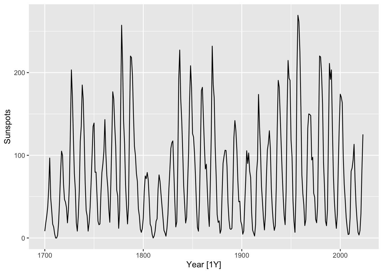
Sunspots are regions of the Sun’s surface that appear temporarily darker than the surrounding areas. They have been studied by astronomers since ancient times, and their frequency is known to have approximately periodic behavior, with a period of about 11 years. In the following figure, we plot the mean daily total sunspot number for each year between 1700 and 2023.
sunspots <- read_rds("_data/cleaned/sunspots.rds")
sunspots |> autoplot(Sunspots)
In view of the data’s periodic nature, it seems to make sense to fit a signal plus noise model of the form \[ X_t = \mu + \alpha_1 \cos(\omega t) + \alpha_2 \sin(\omega t) + W_t, \tag{10.1}\] where \(\omega = 2\pi/11\) and \((W_t) \sim WN(0,\sigma^2)\) for an unknown \(\sigma^2\) parameter to be estimated.
sunspots_fit <- sunspots |>
    model(sin_model = TSLM(Sunspots ~ sin(2 * pi * Year / 11) +
                           cos(2 * pi * Year / 11)))
sigma <- sunspots_fit |>
    pluck(1, 1, "fit", "sigma2") |>
    sqrt()
We next plot the fitted values for the model together with a draw of a sample trajectory generated from the model. We also make plots of its residual diagnostics.
set.seed(5209)
sunspots_fit |>
    augment() |>
    mutate(Sample = .fitted + rnorm(nrow(sunspots)) * sigma,
           Observed = sunspots$Sunspots) |>
    rename(Fitted = .fitted) |>
    pivot_longer(cols = c("Fitted", "Observed", "Sample"),
                 values_to = "Number",
                 names_to = "Type") |>
    filter(Year > 1900) |>
    ggplot() +
    geom_line(aes(x = Year, y = Number, color = Type)) +
    scale_color_manual(values = c("Fitted" = "blue", "Observed" = "black", "Sample" = "orange"))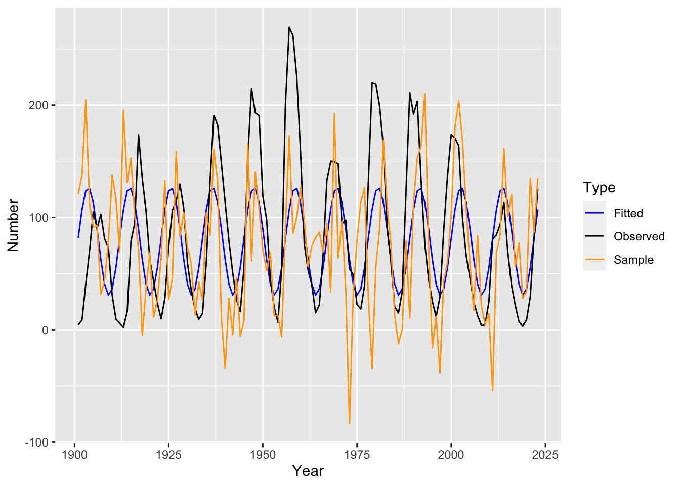
sunspots_fit |>
    gg_tsresiduals()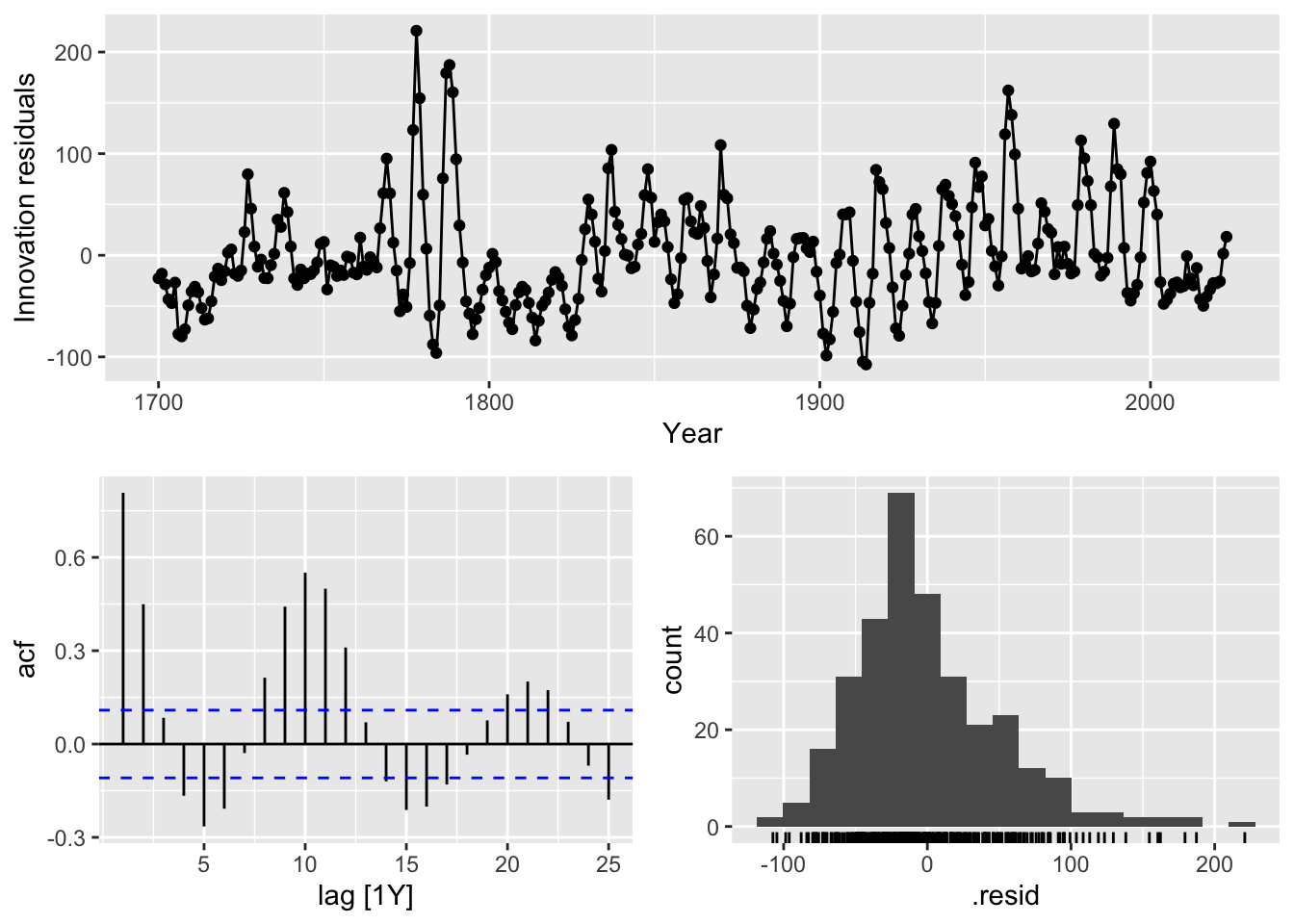
We see that the model residuals do not look like white noise, implying that the model has a poor fit. More precisely, inspecting the fitted values, we observe the following issues:
For this reason, Udny Yule proposed an alternative model that is also based on a single sinusoid, but which incorporates noise in a different way.
Yule’s starting observation was the fact that the mean function of Equation 10.1, \[ x(t) = \mu + \alpha_1 \cos(\omega t) + \alpha_2 \sin(\omega t), \tag{10.2}\] is a solution to the ordinary differential equation (ODE) \[ x''(t) = - \omega^2 \left(x(t) - \mu\right). \tag{10.3}\] Indeed, ODE theory tells us that all solutions to this ODE are of the form Equation 10.2 for some choice of \(\alpha_1\) and \(\alpha_2\) determined by initial conditions.
An ODE tells us how a physical system evolves deterministically based on its inherent properties. For instance, Equation 10.3 is also the ODE governing the small angle oscillation of a pendulum resulting from gravity, which means that the pendulum’s angular position is given by Equation 10.2. The periodic nature of the sunspot data is suggestive of a similar mechanism at work. On the other hand, the departures from pure periodicity suggests that this evolution is not determinstic, but is affected by external noise (which may comprise transient astrophysical phenomena).1 In order to accommodate this, we can add a noise term into Equation 10.3 to get a stochastic differential equation: \[ d^2X_t = - \omega^2 \left(X_t - \mu\right) + dW_t. \] Since time series deals with discrete time points, however, we will first re-interpret Equation 10.3 in a discrete setting.
As seen above, stochastic differential equations are natural generalizations of ODEs, and are used to model complex dynamical systems arising in finance, astrophysics, biology, and other fields. They are beyond the scope of this textbook.
The discrete time analogue of an ODE is a difference equation, which relates the value of a sequence at time \(t\) to its values at previous time points.
Proposition 10.1. The time series Equation 10.2 is the unique general solution to the difference equation: \[ (I-B)^2 x_t = 2(\cos \omega - 1)(x_{t+1} - \mu). \tag{10.4}\]
Here, \(B\) is the backshift operator defined in Chapter 4. Observe the similarity between Equation 10.3 and Equation 10.4, especially bearing in mind that the difference operator \(I-B\) can be thought of as discrete differentiation.
Following the argument in Section 10.1.3, Yule (1927) proposed the model: \[ (I-B)^2 X_t = 2(\cos \omega - 1)(X_{t-1} - \mu) + W_t, \tag{10.5}\] where \((W_t) \sim WN(0,\sigma^2)\). The parameters to be estimated are \(\omega\), \(\mu\), and \(\sigma^2\). In other words, at each time point, the second derivative is perturbed by an amount of exogenous (external) noise.
Note that Equation 10.5 can be rewritten as \[ X_t = \alpha + 2\cos \omega X_{t-1} - X_{t-2} + W_t, \] with \(\alpha = 2(1-\cos\omega)\mu\). In other words, \(X_t\) is a linear combination of its previous two values together with additive noise. It is an example of an autoregressive model of order 2, which we will soon formally define.
We now fit the model and plot both its one-step ahead fitted values \(\hat X_{t|t-1}\) as well as a sample trajectory generated from the model. As before, we also make plots of its residual diagnostics.
sunspots_fit <- sunspots |>
    model(ar_model = AR(Sunspots ~ order(2)))
sigma <- sunspots_fit |>
    pluck(1, 1, "fit", "sigma2") |>
sqrt()set.seed(5209)
sunspots_fit |>
augment() |>
mutate(Sample = sim_ar(sunspots_fit),
Observed = sunspots$Sunspots) |>
rename(Fitted = .fitted) |>
pivot_longer(cols = c("Fitted", "Observed", "Sample"),
values_to = "Number",
names_to = "Type") |>
filter(Year > 1900) |>
ggplot() +
geom_line(aes(x = Year, y = Number, color = Type)) +
scale_color_manual(values = c("Fitted" = "blue", "Observed" = "black", "Sample" = "orange"))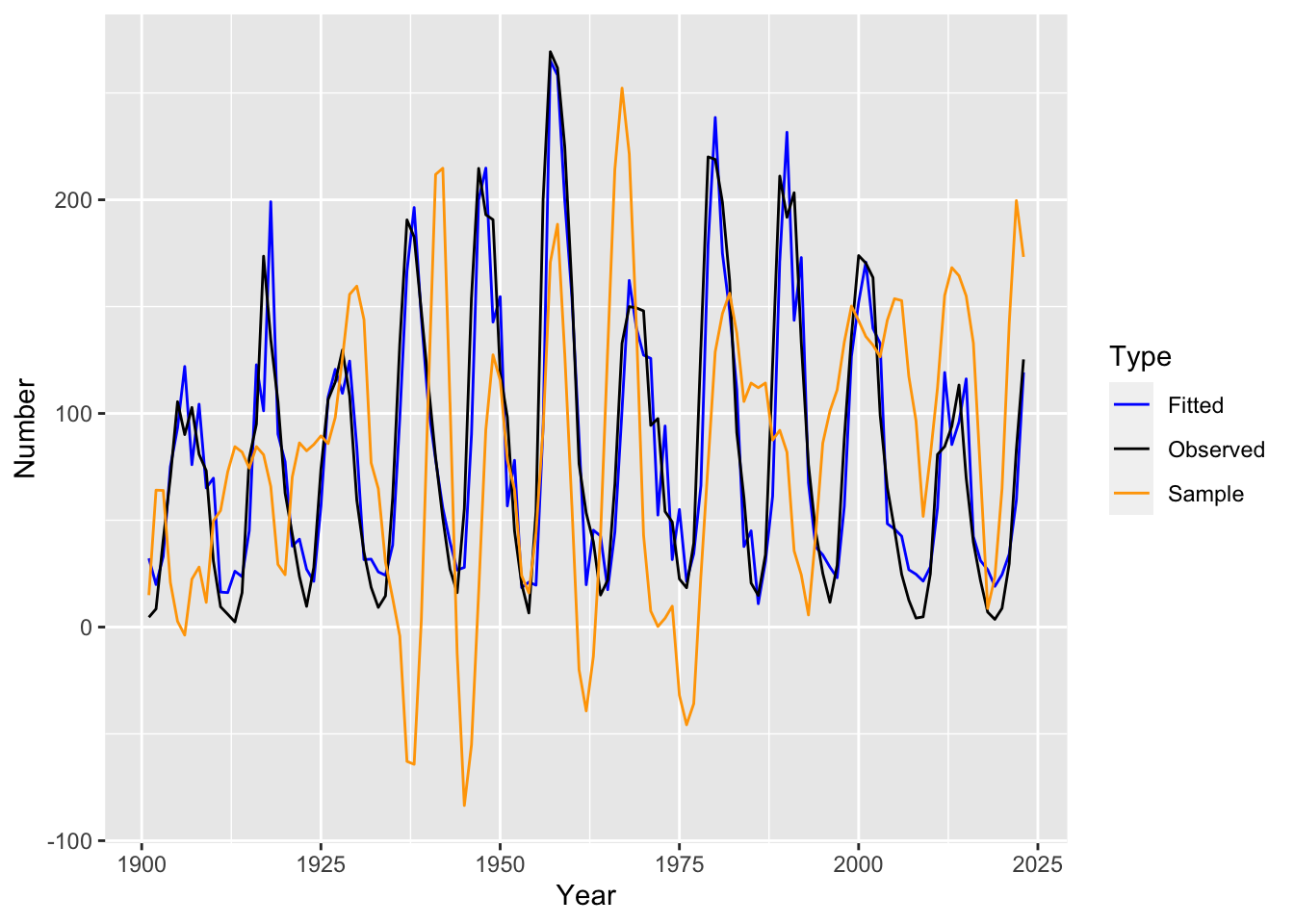
sunspots_fit |>
    gg_tsresiduals()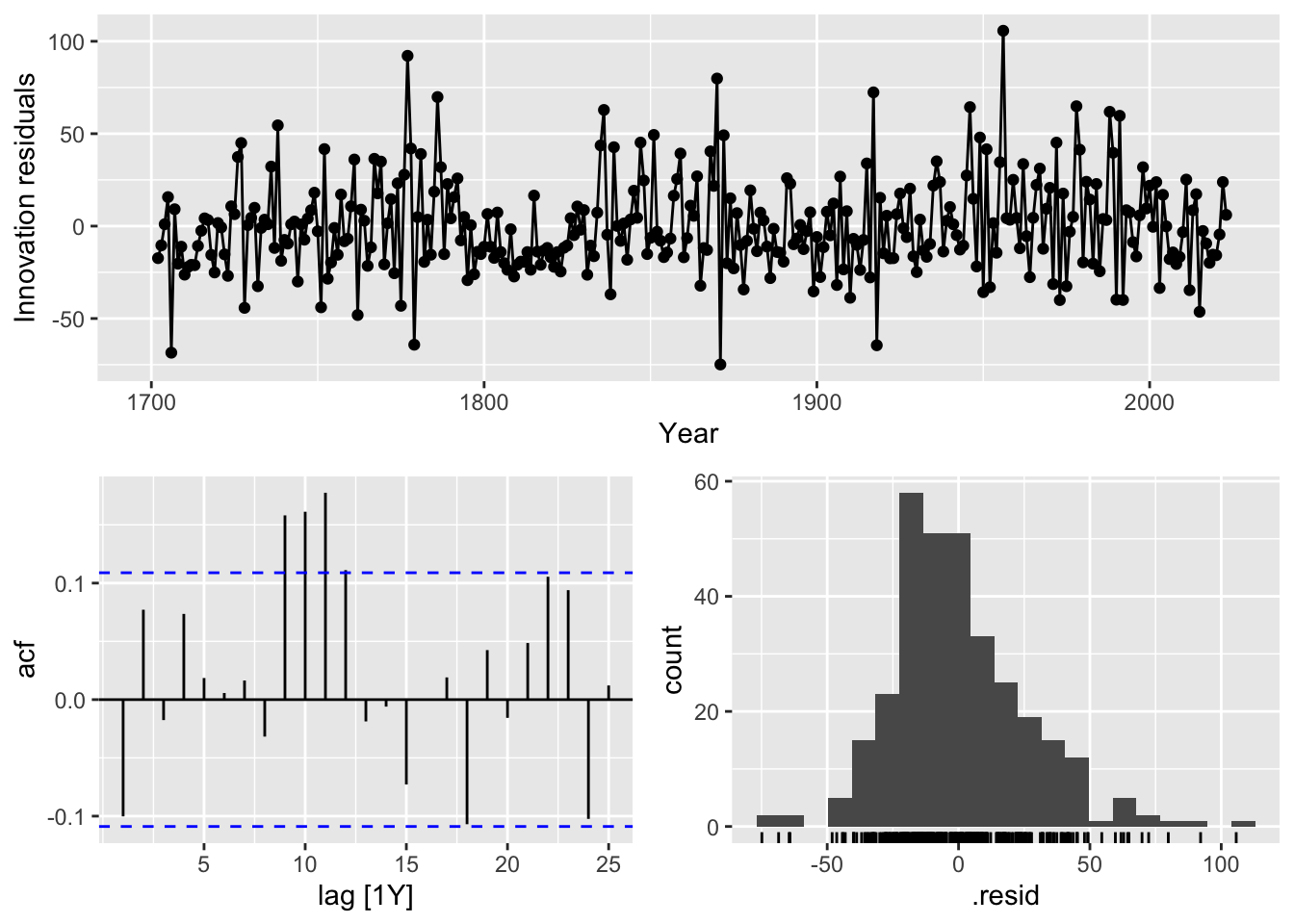
We see that the residuals look much closer to white noise than those of the signal plus noise model, although there still seems to be some remaining outlier values as well as periodic behavior. Furthermore, the fitted values are much closer to the observed time series, and a sample trajectory from the model now seems qualitatively similar to the observed time series.
We have seen that Yule’s model gives a much better fit to the data than the signal plus noise model. As a final comparison between the two models, observe that we can rewrite each model as a pair of equations. First, using Proposition 10.1, the signal plus noise model is equivalent to the following: \[ (I-B)^2 Y_t = 2(\cos \omega - 1)(Y_{t-1} - \mu) \] \[ X_t = Y_t + W_t. \] Meanwhile, Yule’s model is trivially equivalent to: \[ (I-B)^2 Y_t = 2(\cos \omega - 1)(Y_{t-1} - \mu) + W_t \] \[ X_t = Y_t. \]
In both cases, we can think of \(Y_t\) as defining the true state of nature at time \(t\), whose values directly affect its future states. Meanwhile, \(X_t\) reflects the our observation of nature at time \(t\). The signal plus noise model postulates a deterministic evolution of the true state, but introduces observational noise. On the other hand, Yule’s model postulates noiseless observations, but allows for a noisy evolution of the state of nature. It is possible to incorporate both sources of noise in the same model. We will discuss this further when we cover state space models.
An autoregressive model of order \(p\), abbreviated \(\textnormal{AR}(p)\), is a stationary stochastic process \((X_t)\) that solves the equation \[ X_t = \alpha + \phi_1 X_{t-1} + \phi_2 X_{t-2} + \cdots + \phi_p X_{t-p} + W_t, \tag{10.6}\] where \((W_t) \sim WN(0,\sigma^2)\), and \(\phi_1, \phi_2,\ldots,\phi_p\) are constant coefficients.
It is similar to a regression model, except that the regressors are copies of the same time series variable, albeit at earlier time points, hence the term autoregressive.
Note that a simple rearrangement of Equation 10.6 shows that it is equivalent to \[ X_t - \mu = \phi_1 (X_{t-1} - \mu) + \phi_2 (X_{t-2} - \mu) + \cdots + \phi_p (X_{t-p} - \mu) + W_t, \] where \(\mu = \alpha/(1- \phi_1 - \phi_2 - \cdots \phi_p)\). We will soon see that this implies that the mean of \((X_t)\) is \(\mu\). It also implies that centering an autoregressive model does not change its coefficients.
The autoregressive polynomial of the model Equation 10.6 is \[ \phi(t) = 1 - \phi_1 t - \phi_2 t^2 - \cdots - \phi_p t^p. \] Using this notation, we can rewrite Equation 10.6 as \[ \phi(B)X_t = W_t, \] where \(B\) is the backshift operator. Note that for any integer \(k\), \(B^k\) is the composition of the backshift operator \(B\) with itself \(k\) times. Since \(B\) shifts the sequence forwards by one time unit, this resulting operator therefore shifts a sequence forwards by \(k\) time units.
More formally, we can regard \(B\) as an operator on the space of doubly infinite sequences \(\ell^\infty(\Z)\). In other words, it is a linear mapping from \(\ell^\infty(\Z)\) to itself. Mathematically, we say that the space of operators form an algebra. Operators can be added and multiplied like vectors: The resulting operator just outputs the sum or scalar multiple of the original outputs. They can also be composed as discussed earlier.
Introducing this formalism turns out to be quite useful. Apart from allowing for compact notation, the properties of the autoregressive polynomial \(\phi\), in particular its roots and inverses, turn out to be intimately related to properties of the \(\textnormal{AR}(p)\) model.
It is important to understand that Equation 10.6 and its variants are equations and that the model is defined as a solution to equation. A priori, such a solution may not exist at all, or there may be multiple solutions.
We illustrate some of the basic properties of autoregressive models by studying its simplest version, \(\textnormal{AR}(1)\). This is defined via the equation \[ X_t = \phi X_{t-1} + W_t, \tag{10.7}\] where \((W_t) \sim WN(0,\sigma^2)\).2 It is convention to slightly abuse notation, using \(\phi\) to denote both the AR polynomial and its coefficient. The meaning will be clear from the context.
Proposition 10.1 (Existence and uniqueness of solutions). Suppose \(|\phi| < 1\), then there is a unique stationary solution to Equation 10.7. This solution is a causal linear process.
Proof. We first show existence. Consider the expression \[ X_t \coloneqq \sum_{j=0}^\infty \phi^j W_{t-j}. \tag{10.8}\] Since \[ \sum_{j=0}^\infty |\phi^j| = \frac{1}{1-|\phi|} < \infty, \] the expression converges absolutely, so \(X_t\) is well-defined. Indeed this is a causal linear process, and is in particular stationary. It is also easy to see that it satisfies Equation 10.7: \[ \begin{split} \phi X_{t-1} + W_t & = \phi\left(\sum_{j=0}^\infty \phi^j W_{t-1-j}\right) + W_t \\ & = \sum_{j=0}^\infty \phi^{j+1} W_{t-1-j} + W_t \\ & = \sum_{k=1}^\infty \phi^{k} W_{t-k} + W_t \\ & = X_t. \end{split} \]
To see that it is unique, suppose we have another stationary solution \((Y_t)\). We may then use Equation 10.7 to write \[ \begin{split} Y_t & = \phi Y_{t-1} + W_t \\ & = \sum_{j=0}^l \phi^j W_{t-j} + \phi^l Y_{t-l}, \end{split} \] where the second equality holds for any integer \(l > 0\). We thus see that for the same white noise sequence, we have \[ Y_t - Z_t = \sum_{l+1}^\infty \phi^j W_{t-j} + \phi^l Y_{t-l}. \] We can obtain a variance bound on the right hand side that tends to 0 as \(l \to \infty\): \[ \begin{split} \Var\left\lbrace \sum_{j=l+1}^\infty \phi^j W_{t-j} + \phi^l Y_{t-l} \right\rbrace & \leq 2\Var\left\lbrace \sum_{j=l+1}^\infty \phi^j W_{t-j}\right\rbrace + 2\Var\left\lbrace \phi^l Y_{t-l}\right\rbrace \\ & = \frac{2\phi^{2l}\sigma^2}{1-\phi^2} + \phi^{2l}\gamma_Y(0). \end{split} \] Since the left hand side is independent of \(l\), we get \(Y_t =_d Z_t\) as we wanted. \(\Box\)
This theorem allows us to speak of the solution to Equation 10.7, and we sometimes informally refer to the equation as the model. As such, we also refer to Equation 10.7 for \(|\phi| < 1\) as a causal \(\textnormal{AR}(1)\) model.
Proposition 10.2 (Mean, ACVF, ACF). Let \((X_t)\) be the solution to Equation 10.7. Then We have \(\mu_X = 0\) and \[ \gamma_X(h) = \frac{\sigma^2\phi^h}{1-\phi^2}, \] \[ \rho_X(h) = \phi^h \] for all \(h \in \mathbb{Z}\).
Proof. Using Equation 10.8, we get \[ \mu_X = \E\left\lbrace \sum_{j=0}^\infty \phi^j W_{t-j} \right\rbrace = \sum_{j=0}^\infty \phi^j \E\left\lbrace W_{t-j} \right\rbrace = 0. \] Next, using Equation 9.4, we get \[ \gamma_X(h) = \sigma^2 \sum_{j=0}^\infty \phi^j \phi^{j+h} = \frac{\sigma^2\phi^h}{1-\phi^2}. ~\Box \]
We thus see that the ACF has an exponential decay.
The recurrence form of Equation 10.7 makes forecasting extremely straightforward. Recall that we are interested in both distributional and point forecasts (see Section 7.9). Given a statistical model and observations \(x_1,x_2,\ldots,x_n\) drawn from the model, the distributional forecast for a future observation \(X_{n+h}\) is just its conditional distribution given our observed values: \[ \P\left\lbrace X_{n+h} \leq x_{n+h}|X_1 = x_1, X_2 = x_2,\ldots,X_n = x_n \right\rbrace. \tag{10.9}\]
Given an \(\textnormal{AR}(1)\) model with a further assumption of Gaussian white noise, the distributional forecast is extremely easy to derive. We simply recursively apply Equation 10.7 to get \[ X_{n+h} = W_{n+h} + \phi W_{n+h-1} + \cdots + \phi^{h-1}W_{n+1} + \phi^hX_n. \] Since \(W_{n+1},\ldots,W_{n+h}\) are independent of \(X_1,X_2,\ldots,X_n\), this means that Equation 10.9 is simply \(N\left(\phi^h x_n, \frac{(1-\phi^{2h})\sigma^{2}}{1-\phi^2} \right)\). In particular, we get \[ \hat x_{n+h|n} = \phi^h x_n \] and a prediction interval at the 95% level is \[ (\phi^h x_n - 1.96v_h^{1/2} , \phi^h x_n + 1.96v_h^{1/2}), \] where \(v_h = \frac{(1-\phi^{2h})\sigma^{2}}{1-\phi^2}\).
Note that as the forecast horizon \(h\) increases, the point forecast converges to \(\mu_X = 0\), while the variance of the forecast distribution increases to \(\gamma_X(0) = \sigma^2/(1-\phi^2)\). In other words, the forecast distribution converges to the marginal distribution of \(X_t\) (for any \(t\)), and we see that our observations become increasingly irrelevant as we forecast further out into the future.
In the plot below, we create sample trajectories from \(\textnormal{AR}(1)\) models with \(\phi\) set to be \(0.3\), \(0.9\) and \(-0.9\) (from top to bottom). We also show the distributional forecasts up to the horizon \(h=20\).
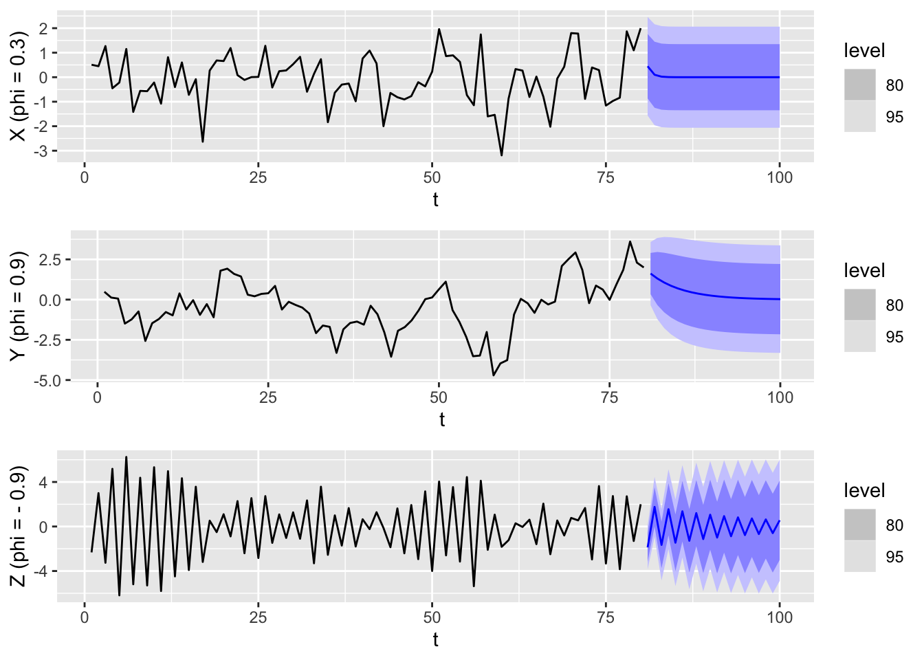
We see that \(\phi\) has a strong effect on both the shape of the trajectory as well as the forecasts. When \(\phi\) is small and positive, then the trajectory looks similar to that of white noise, whereas when \(\phi\) is large and positive, there are fewer fluctuations, and it looks similar to a random walk. The point forecasts also decay more slowly towards the mean. Finally, when \(\phi\) is negative, consecutive values are negatively correlated, which results in rapid fluctuations.
If we assume that the white noise in Equation 10.7 is Gaussian, then the resulting \(\textnormal{AR}(1)\) process is also a Gaussian process, which means that its distribution is fully determined by its mean and ACVF functions. Note that the ACVF function of any stationary process is even: \(\gamma_X(h) = \gamma_X(-h)\). This means the covaraince matrix of \((X_1,X_2,\ldots,X_n)\), \(\Gamma_{1:n} = (\gamma_X(i-j))_{ij=1}^n\), is symmetric and so the distribution of \((X_1,X_2,\ldots,X_n)\) is the same as that of its time reversal \((X_n,X_{n-1},\ldots,X_1)\). In summary, stationary \(\textnormal{AR}(1)\) processes are reversible, and we cannot tell the direction of time simply by looking at a trajectory.
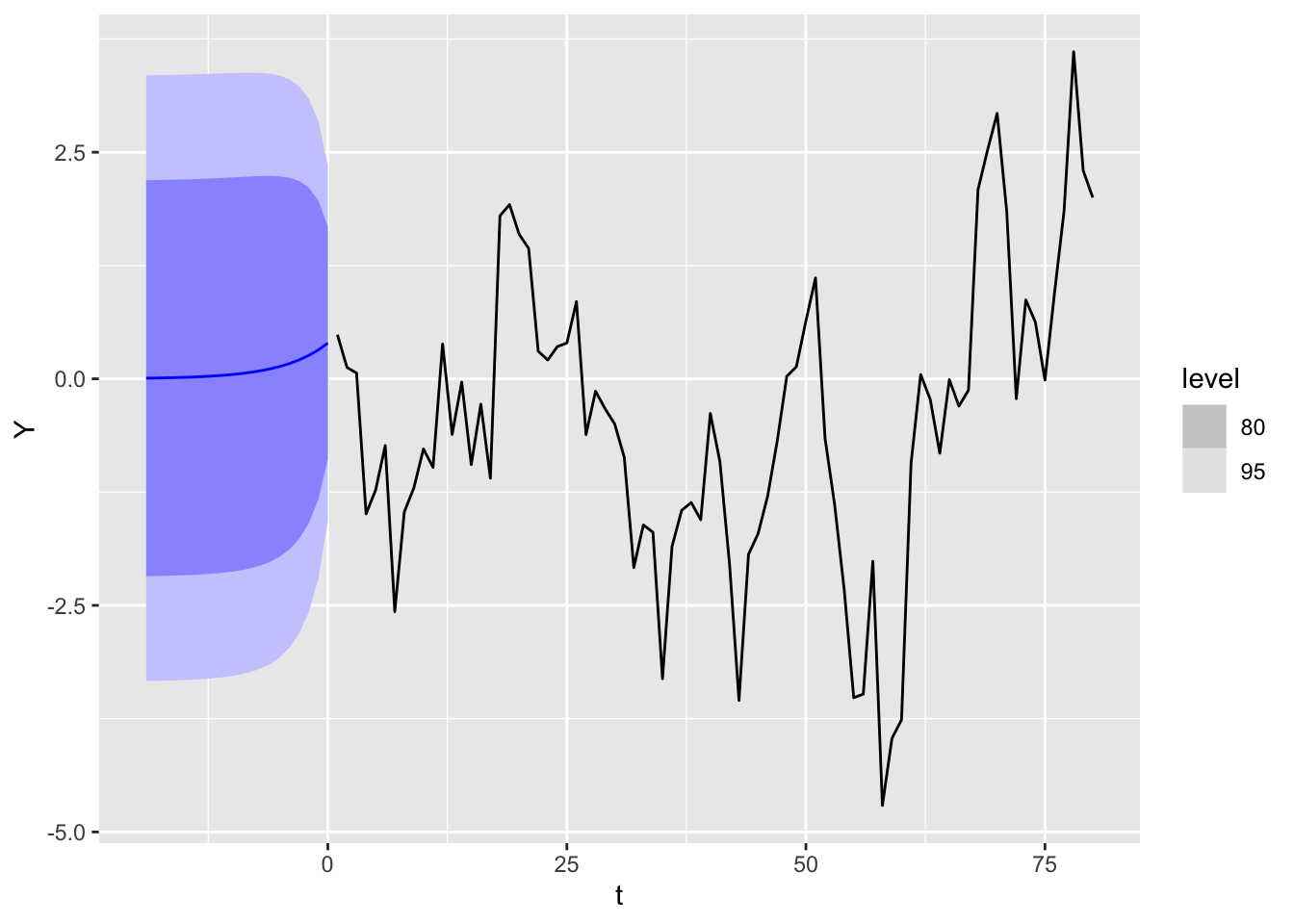
Many real world time series are not reversible, which means that \(\textnormal{AR}(1)\) models (and linear processes more generally) are poor fits whenever this holds. On the other hand, reversibility allows us to easily perform backcasting, which is the estimation of past values of a time series that are unknown.
An \(\textnormal{AR}(1)\) model only has two parameters: \(\phi\) and \(\sigma^2\). Given observed data \(x_1,x_2,\ldots,x_n\), we may estimate these parameters as follows. First, Proposition 10.2 tells us that \(\phi = \rho_X(1)\), so we may use the estimator \(\hat\phi \coloneqq \hat\rho_X(1)\). Substituting this into Theorem 9.2 then gives \[ \sqrt n (\hat\phi - \phi) \to N(0,1-\phi^2). \]
Since \(\sigma^2 = \gamma_X(0)(1-\phi^2)\), we may estimate \[ \hat\sigma^2 \coloneqq \hat\gamma_X(0)(1 - \hat\rho_X(1)^2) = \hat\gamma_X(0) - \hat\gamma_X(1)^2/\hat\gamma_X(0). \] Since the sample ACVF is consistent (Theorem A.6 in Shumway and Stoffer (2000)), so is this estimator.
Explosive solution. If a choice of \(|\phi| < 1\) results in a unique stationary solution, what happens when \(|\phi| > 1\)? If we start with a fixed initial value \(X_0 = c\), we can iterate Equation 10.7 to get \[ X_t = \sum_{j=1}^t \phi^j W_j + \sum_{j=1}^t \phi^j c. \] The mean function is thus \(\mu_X(t) = \sum_{j=1}^t \phi^j c\), while the marginal variance is given by \[ \mu_X(t, t) = \Var\left\lbrace \sum_{j=1}^t \phi^j W_j\right\rbrace = \frac{(\phi^{2t}-1)}{\phi^2 - 1}. \] Both values diverge to infinity exponentially as \(t\) increases. The resulting time series model is sometimes called an explosive \(\textnormal{AR}(1)\) process. In particular, it is not stationary.
The above is probably unsurprising. When \(\phi = 1\), then Equation 10.7 is the defining equation for a random walk, which we already know is non-stationary. It is therefore somewhat unintuitive that there exist unique stationary solutions to Equation 10.7 when \(|\phi| > 1\).
Stationary solution. Define the expression \[ X_t \coloneqq -\sum_{j=1}^\infty \phi^{-j}W_{t+j}. \tag{10.10}\] Using the same arguments as in the proof of Proposition 10.1, one can check that this converges absolutely, and that \((X_t)\) is stationary and satisfies Equation 10.7. Indeed, it is the unique such solution. On the other hand, this solution doesn’t make physical sense because \(X_t\) depends on the future innovations \(W_{t+1}, W_{t+2},\ldots\).3 Formally, we say that such a solution is non-causal, unlike Equation 10.8.
Because of the the problems of these two solutions, Equation 10.7 with \(|\phi| > 1\) is rarely used for modeling.
One may calculate the ACVF of Equation 10.10 to be \[ \gamma_X(h) = \frac{\sigma^2\phi^{-2}\phi^{-h}}{1-\phi^{-2}}. \] This is the same as that of a causal \(\textnormal{AR}(1)\) process with noise variance \(\tilde\sigma^2 \coloneqq \sigma^2\phi^{-2}\) and coefficient \(\tilde\phi \coloneqq \phi^{-1}\). If we assume Gaussian white noise, this implies that the two time series models are the same.
We now generalize our findings about \(\textnormal{AR}(1)\) models to general \(\textnormal{AR}(p)\) models. Along the way, we will see that while the flavor of the results remains consistent, the technical difficulty of the tools we need increases sharply.
Theorem 10.3 (Existence and uniqueness of solutions) Let \(\phi(z)\) be the autoregressive polynomial of Equation 10.6. Suppose \(\phi(z) \neq 0\) for all \(|z| \neq 1\), then Equation 10.6 admits a unique stationary solution. If futhermore \(\phi(z) \neq 0\) for all \(|z| \leq 1\), then the solution is causal and has the form \[ X_t = \sum_{j=0}^\infty \psi_j W_{t-j}, \] where \[ \phi(z) \cdot \left(\sum_{j=0}^\infty \psi_j z^j \right) = 1. \]
Exactly what this noise comprises of seems to be a topic of current research.↩︎
We omit the constant term in the equation due to our remarks in the previous section.↩︎
Because of this lack of independence, we cannot use the equations in Section 10.3.3 to forecast or simulate sample trajectories.↩︎