We have previously motivated \(\textnormal{AR}(p)\) models as describing noisy dynamical systems, that is, where each value \(X_t\) is determined by its previous values according to some natural law, but this evolution is perturbed by some external noise \(W_t\). This model makes an underlying assumption that \(X_t\) is the true state of nature. However, in many situations, it is more realistic to assume that we observe measurements that are corrupted by noise. In this case, we may formulate a (linear) state space model, which can be written as the following pair of equations.
Equation 13.1 is called the state equation, while Equation 13.2 is called the observation equation. Here, each \(X_t \in \R^p\) is an unobserved random vector modeling the state of nature, \(\Phi\) is a fixed matrix that governs the evolution of the system, \(Y_t \in \R^q\) is the observed data vector, \(A_t\) is called the observation matrix, while \(W_t\) and \(V_t\) are mean zero random vectors to be thought of as noise. We usually model \(W_t\) and \(V_t\) as Gaussian random vectors, in which case \((X_t,Y_t)\) is a Gaussian process.
Equation 13.1 and Equation 13.2 together produce an extremely flexible model class that subsumes most of the models we have seen so far as special cases. In addition to allowing for measurement error, the vector forms of the state and observation variables allows us to simultaneously model multiple related time series. Furthermore, while these equations seem to incorporate only one lag, we can use them to model multiple time lags via a simple vectorization trick:1
Finally, using appropriate choices for \(A_t\), we can easily model missing data.
Note
The state equation is a Markov chain, which means that the state space model can be said to be a hidden Markov Model. However, by convention, the term “hidden Markov model” is used to describe models with discrete state spaces, while the term “state space model” is used to describe models with continuous state spaces.
13.2 Examples
Before proceeding further, we first introduce a few examples of time series data for which a state space model is particularly useful.
13.2.1 Global temperature
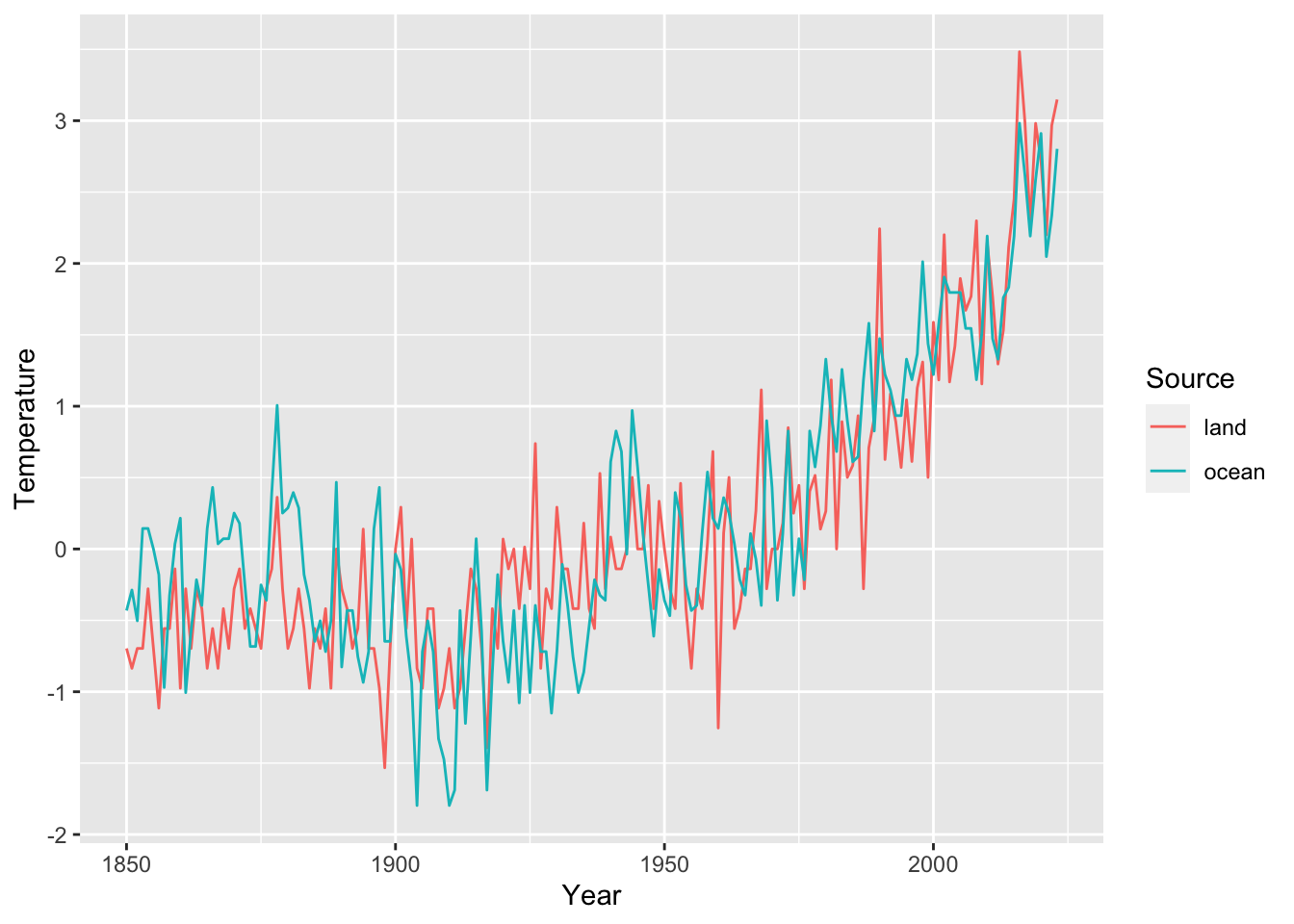
The astsa package contains two time series measuring annual global temperature deviations.
gtemp_land: This measures temperatures averaged over the Earth’s land area.
gtemp_ocean: This measures temperatures averaged over the Earth’s sea surface.
Figure 13.1: Annual global temperature deviations, measured in Celsius, with respect to the the 1991-2020 average.
The two time series, which we denote by \((Y_{t1})\) and \((Y_{t2})\), are not independent, but when suitably normalized, can be thought of as noisy measurements of an underlying “true” temperature of the Earth \((X_t)\). Modeling \((X_t)\) as a random walk with drift, we get the following pair of equations.
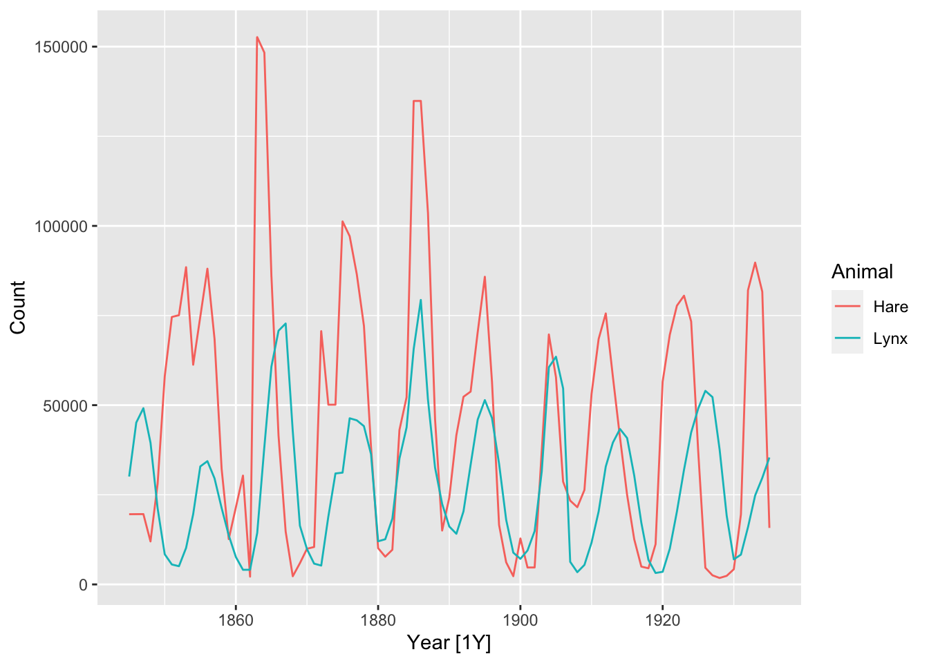
Figure 13.2: Hudson Bay Company trading records for Snowshoe Hare and Canadian Lynx furs from 1845 to 1935.
The trading records are obviously proxies for the true unobserved population size of both species living in the area during each year, which denote as \((X_{t1})\) and \((X_{t2})\). Since both species interact via predation, it is natural to model their dynamics using a vector autoregressive (VAR) model: \[
\left[
\begin{matrix}
X_{t1} \\
X_{t2}
\end{matrix}
\right] =
\left[
\begin{matrix}
\phi_{11} & \phi_{12} \\
\phi_{21} & \phi_{22}
\end{matrix}
\right]
\left[
\begin{matrix}
X_{t-1,1} \\
X_{t-1,2}
\end{matrix}
\right] +
\left[
\begin{matrix}
W_{t1} \\
W_{t2}
\end{matrix}
\right].
\] For the observation equation, we have: \[
\left[
\begin{matrix}
Y_{t1} \\
Y_{t2}
\end{matrix}
\right] =
\left[
\begin{matrix}
\beta_{t1} & 0 \\
0 & \beta_{t2}
\end{matrix}
\right]
\left[
\begin{matrix}
X_{t,1} \\
X_{t,2}
\end{matrix}
\right] +
\left[
\begin{matrix}
P_{t1} \\
P_{t2}
\end{matrix}
\right].
\] Here, \(\beta_{t1}\) and \(\beta_{t2}\) model the percentage of each population that was hunted during that year.
13.2.3 Biomarker monitoring
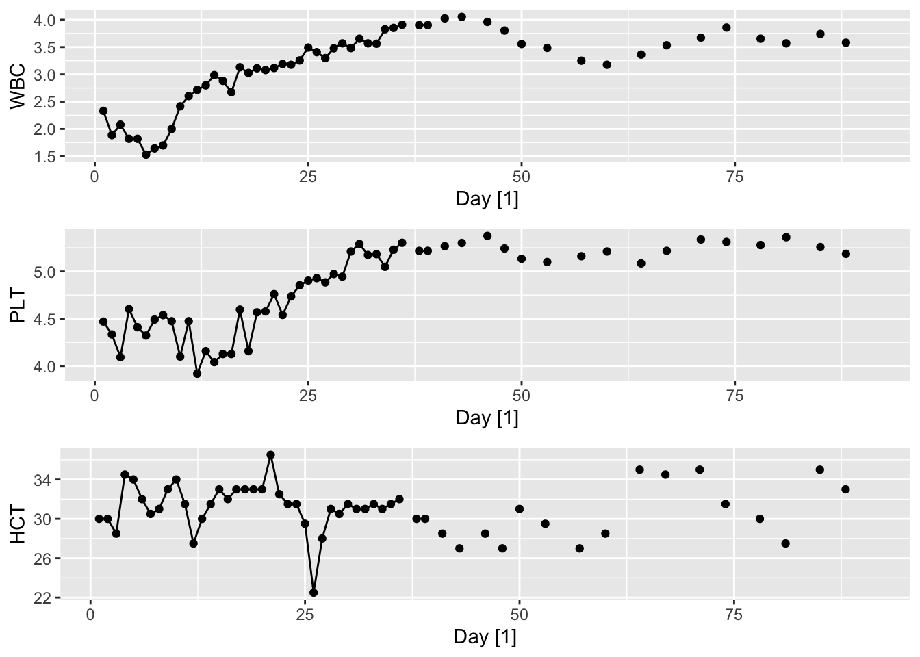
The following dataset measures the log white blood count (WBC), log platelet count (PLT), and hematocrit (HCT) for a cancer patient for 91 days after undergoing a bone marrow transplant.
Figure 13.3: Monitored blood biomarkers for a cancer patient.
Let us denote the three blood biomarkers as \((X_{t1}, X_{t2}, X_{t3})\). Here, we have a high density of missing values, especially after the first 35 days. The goal is to impute the missing values, in which case, we may use the state equation Equation 13.1 and an observation equation Equation 13.2 with \(A_t\) equal to the identity matrix if a blood sample was taken on that day and equal to the zero matrix otherwise.
13.2.4 Object tracking
One of the earliest applications of state space models was to the problem of tracking spacecraft. The goal of the Apollo program in the 1960s was to send a manned spacecraft to the moon and back, and one of the challenges was being able to make the spacecraft follow a precisely calculated trajectory. However, the spacecraft was subject to unpredictable forces, which may result in uncertain dynamics. This could be corrected if we knew how far the spacecraft was deviating from the trajectory, but the instruments on board the spacecraft could only produce noisy measurements at irregular intervals.
Such a set-up can be modeled using the Gaussian linear model. We show the equations in 2 spatial dimensions for simplicity. Here, \(X_t \in \R^4\) records the position and velocity in the two coordinates, and we assume that measurements are taken at intervals of \(\delta\) seconds.
Previously, we have focused on time series forecasting as the primary inferential task of time series analysis. The state space formulation means that estimating the unobserved latent state \(X_t\) is also of interest.
There are three versions of this, depending on the relationship of the time index of interests, \(t\), to the indices of the observed data \(Y_1,Y_2,\ldots,Y_s\). We give the tasks different names:
Smoothing: This is when \(s > t\), i.e. we want to estimate a previous latent state.
Filtering: This is when \(s=t\), i.e. we want to estimate the current latent state.
Forecasting: This is when \(s < t\), i.e. we want to estimate a future latent state.
Similar to our previous discussion, we are interested in both point prediction and prediction intervals. Since we assume a Gaussian model, best linear prediction is the same as conditional means. In other words, \[
\hat X_{t|s} \coloneqq \E\lbrace X_t | Y_1,Y_2,\ldots Y_s\rbrace
\tag{13.3}\] is equal to the best linear prediction of \(X_t\) given \(Y_1,Y_2,\ldots Y_s\).
13.3.2 The Kalman filter
We have seen how to calculate conditional distributions for Gaussian distributions. If we assume in addition that \((W_t)\) and \((V_t)\) are each i.i.d as well as independent of each other, the calculations simplify into a relatively simple set of equations, which are together known as the Kalman filter.
Proposition 13.1.(Kalman filter) The following equations hold:
Updating state index: \[
\hat X_{t|t-1} = \Phi \hat X_{t-1|t-1},
\tag{13.4}\]\[
P_{t|t-1} = \Phi P_{t-1|t-1} \Phi^T + Q.
\tag{13.5}\]Updating observation index: \[
\hat X_{t|t} = \hat X_{t|t-1} + K_t(Y_t - A_t \hat X_{t|t-1}),
\tag{13.6}\]\[
P_{t|t} = (I - K_tA_t)P_{t|t-1},
\tag{13.7}\] where \[
K_t \coloneqq P_{t|t-1} A_t^T \left(A_t P_{t|t-1}A_t^T + R\right)^{-1}
\tag{13.8}\] is called the Kalman gain.
Proof.Equation 13.4 follows from applying the BLP operator to both sides of Equation 13.1 and using linearity, similar to our derivation of recursive forecasting for \(\textnormal{AR}(p)\) models. To get Equation 13.5, we use the independence of \(W_t\) and \(Y_1,Y_2,\ldots,Y_{t-1}\) to get \[
\begin{split}
P_{t|t-1} & = \Cov\lbrace X_t | Y_1,Y_2,\ldots,Y_{t-1}\rbrace \\
& = \Cov\lbrace \Phi X_{t-1} + W_t | Y_1,Y_2,\ldots,Y_{t-1}\rbrace \\
& = \Cov\lbrace \Phi X_{t-1} | Y_1,Y_2,\ldots,Y_{t-1}\rbrace + \Cov\lbrace W_t | Y_1,Y_2,\ldots,Y_{t-1}\rbrace \\
& = \Phi P_{t-1|t-1}\Phi^T + Q.
\end{split}
\]
To prove Equation 13.6 and Equation 13.7, we need to compute the joint conditional distribution of \(X_t\) and \(Y_t\) given \(Y_1,\ldots,Y_{t-1}\). The conditional covariance of \(X_t\) and \(Y_t\) is: \[
\begin{split}
\Cov\lbrace X_t, Y_t | Y_1,\ldots,Y_{t-1}\rbrace & = \Cov\lbrace X_t, A_t X_t + V_t | Y_1,\ldots,Y_{t-1}\rbrace \\
& = \Cov\lbrace X_t | Y_1,Y_2,\ldots,Y_{t-1}\rbrace A_t^T \\
& = P_{t|t-1}A_t^T.
\end{split}
\] Meanwhile, the conditional covariance of \(Y_t\) is: \[
\begin{split}
\Cov\lbrace Y_t | Y_1,\ldots,Y_{t-1}\rbrace & = \Cov\lbrace A_t X_t + V_t | Y_1,\ldots,Y_{t-1}\rbrace \\
& = \Cov\lbrace A_t X_t | Y_1,Y_2,\ldots,Y_{t-1}\rbrace + \Cov\lbrace V_t | Y_1,Y_2,\ldots,Y_{t-1}\rbrace \\
& = A_tP_{t|t-1}A_t^T + R.
\end{split}
\] As such, \[
\left[
\begin{matrix}
X_t \\
Y_t
\end{matrix}
\right] ~\Bigg| ~Y_1,\ldots, Y_{t-1} \sim N\left(
\left[
\begin{matrix}
\hat X_{t|t-1} \\
A_t \hat X_{t|t-1}
\end{matrix}
\right],
\left[
\begin{matrix}
P_{t|t-1} & P_{t|t-1}A^T \\
A_tP_{t|t-1} & A_tP_{t|t-1}A_t^T + R
\end{matrix}
\right]
\right).
\] Now further conditioning on \(Y_t\) and using the formula for conditional distributions, we get \[
X_t ~|~Y_1,\ldots,Y_t \sim N(\hat X_{t|t-1} + K_t(Y_t - A_t \hat X_{t|t-1}), (I-K_tA_t)P_{t|t-1}).
\] The mean and covariance of this distribution gives the formulas for \(\hat X_{t|t}\) and \(P_{t|t}\). \(\Box\)
Applying these equations recursively for \(t=1,2,\ldots\) allows us to perform filtering as well as one-step-ahead forecasting. If we wish to forecast for \(t > n +1\), we may apply the following recursively: \[
\hat X_{t |n} = \Phi\hat X_{t-1|n},
\]\[
P_{t |n} = \Phi P_{t-1|n}\Phi^T + Q.
\]
One needs initial values \(\hat X_{0|0}\) and \(P_{0|0}\) in order to start the recursion. For most real data applications, one can use any reasonable values.
13.3.3 Kalman smoother
In order to perform smoothing, we need a further set of equations.
Proof. The proof of this proposition is fairly technical and is omitted. We refer interested readers to Property 6.2 in Shumway and Stoffer (2000).
To obtain \(\hat X_{t-1|n}\) and \(P_{t-1|n}\), one starts with the values \(\hat X_{n|n}\) and \(P_{n|n}\) obtained via Proposition 13.1, and then applies Equation 13.9 and Equation 13.10 recursively for \(t = n, n-1, \ldots\).
13.3.4 Exogenous variables
In certain settings, rather than simply observing the values of a time series, one is able to exert some control over the underlying dynamical system. For instance, in spacecraft tracking, the trajectory of the spacecraft can be adjusted using its thrusters. In biomarker monitoring, the patient could be administered with certain drugs at various time points.
We can model these inputs as exogenous variables\(U_t\) that are inserted into the state and observation equations as follows: \[
X_t = \Phi X_{t-1} + \Upsilon U_t + W_t,
\]\[
Y_t = A_t X_t + \Gamma U_t + V_t.
\]
Note
Exogenous variables can also be included in AR, ARMA and ARIMA models. In this case, we append an “X” to the model abbreviation, i.e. we call such models ARX, ARMAX and ARIMAX respectively.
13.4 Estimation
We are sometimes able to specify some of the model parameters \(\Phi\), \(A_t\), \(Q\), and \(R\), using prior knowledge. This is the case for the spacecraft tracking example because of the laws of motion as well as known properties of the spacecraft sensors. However, in most other cases, the parameters have to be estimated from the data.
As usual, we may perform maximum likelihood estimation. Given observations \(Y_1 = y_1, Y_2 = y_2,\ldots, Y_n = y_n\), the likelihood to be optimized is2\[
p(\Phi, A, Q, R | y_1,\ldots y_n),
\] which is a Gaussian with known covariance structure. Using calculations similar to those for \(\textnormal{AR}(p)\) models in Chapter 10, we can convert this into to a more convenient form that can be easily differentiated and thus optimized numerically.
The MLE has consistency and asymptotic normality properties (see Property 6.4 in Shumway and Stoffer (2000)).
Since state space models typically have many more parameters compared with ARIMA models, one has to be careful about having enough data to fit these models. It is useful to adopt a Bayesian approach, which allows one to integrate some prior knowledge about the parameters but at the same time allow them to be influenced by the observed data.
13.5 State space modeling in R
Unfortunately, the fable suite of packages does not have state space modeling functionality. The CRAN task view for time series describes a number of packages that can be used. Unfortunately, all packages seem to use different notation for the model parameters. We will use a package called KFAS, which seems to be the most well-established.
More information about the package can be found via its CRAN and github pages.
require(KFAS)
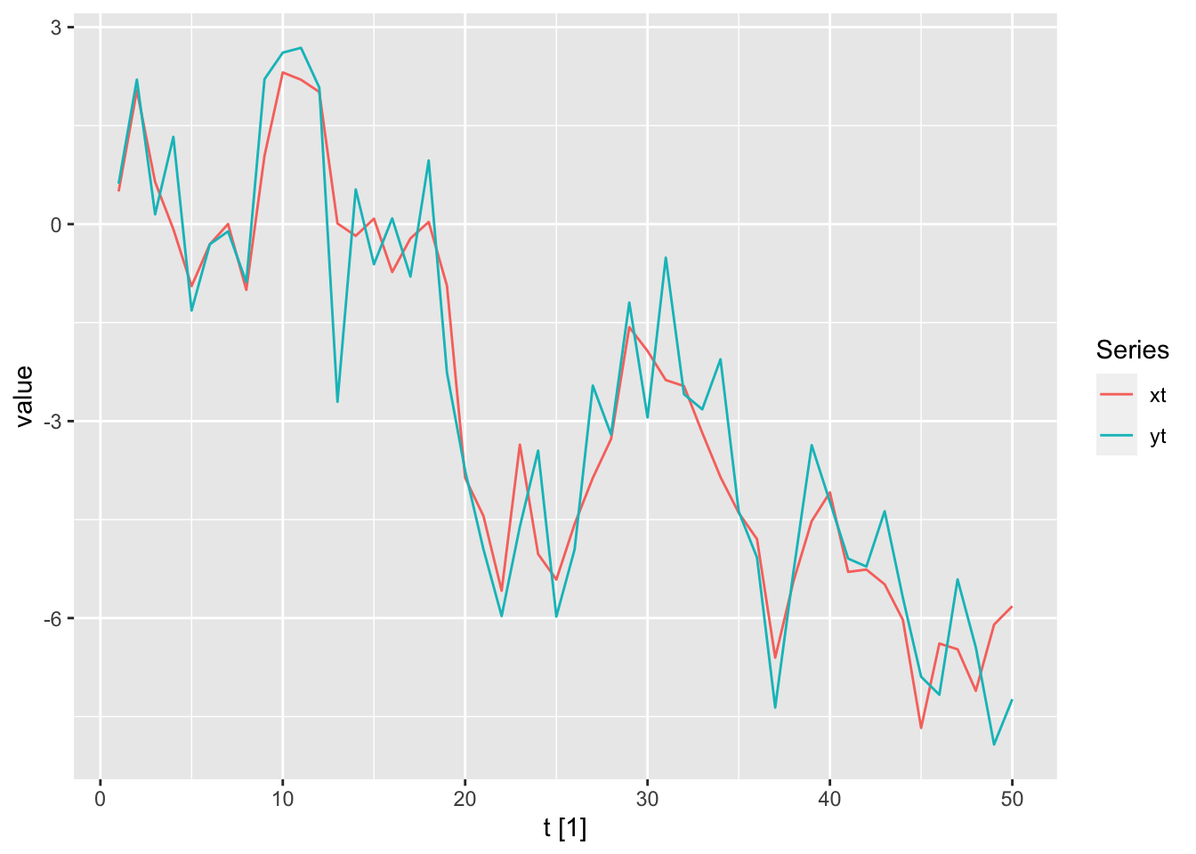
13.5.1 Local level model
A local level model is defined by the equations \[
X_t = X_{t-1} + W_t,
\]\[
Y_t = X_t + V_t.
\] We can interpret this as the time series \((Y_t)\) comprising a “trend” component, modeled as a random walk, and a random component \((V_t)\).
We simulate and plot a draw from this model below.
Figure 13.4: The state (xt) and observation (yt) sequences from a local level model.
We now specify and fit the model using functions from KFAS.
ll_model <-SSModel(as.ts(ll_dat$yt) ~SSMcustom(1Z =1, T =1, R =1, Q =1) -1, H =1)ll_out <-KFS(ll_model, filtering ="state", 2smoothing ="state")ll_dat <-tibble(ll_dat,3forecast = ll_out$a[-(n+1)],filtered = ll_out$att,smoothed = ll_out$alphahat,4forecast_var =drop(ll_out$P)[-(n+1)],filtered_var =drop(ll_out$Ptt),smoothed_var =drop(ll_out$V))
1
This functions SSModel() and SSMcustom() are used to specify the model. Z represents the observation matrix (\(A\)), T represents the state matrix (\(\Phi\)), R represents a matrix applied to the noise vector (\(W_t\)) in the state equation, Q represents the covariance of \(W_t\), and H represents the covaraince of \(V_t\).
2
The function KFS() is used to fit the model.
3
We remove the last time index because it is a forecast for time \(n+1\).
4
We apply drop() to reduce the dimensionality of this sequence. The covariances are usually matrices, but since we have specified the noise to be scalar, these matrices are \(1 \times 1\) in size.
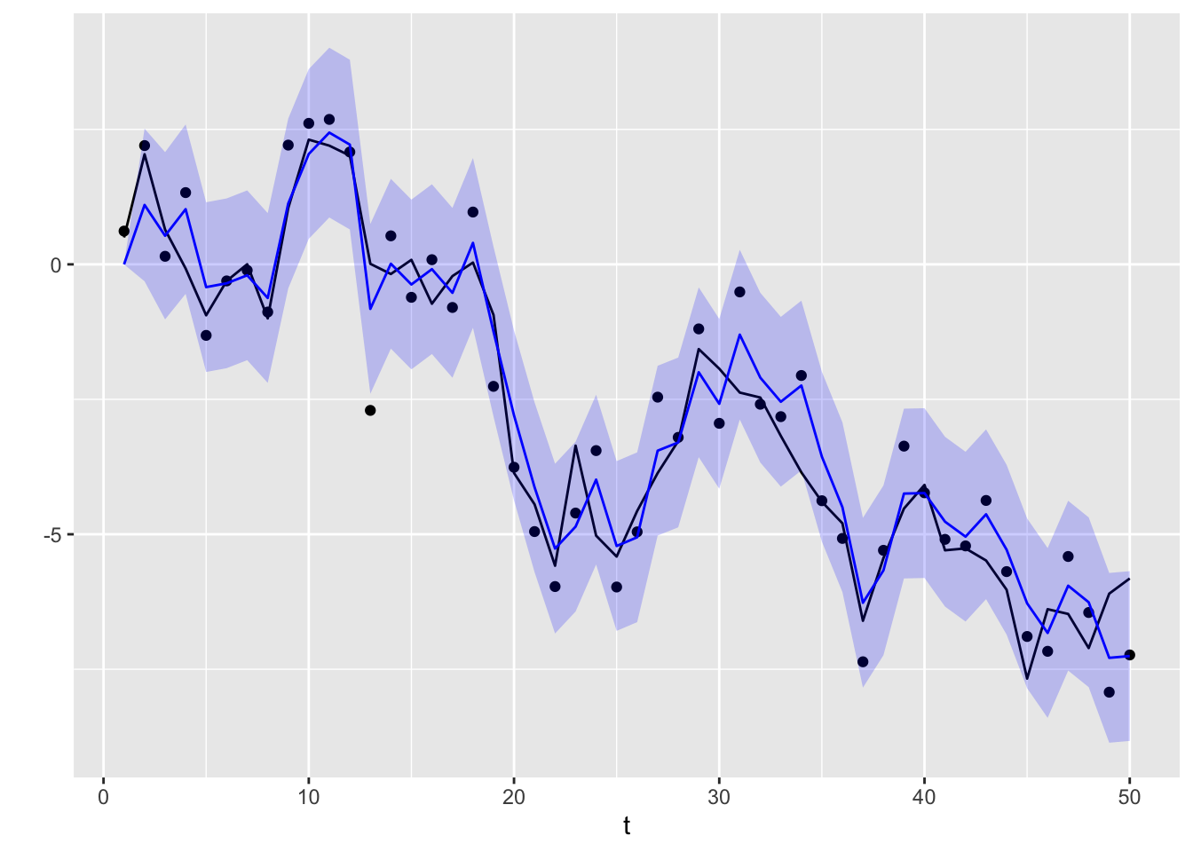
ll_dat |>ggplot(aes(x = t)) +geom_point(aes(y = yt)) +geom_line(aes(y = xt), color ="black") +geom_line(aes(y = forecast), color ="blue") +geom_ribbon(aes(ymin = forecast +2*sqrt(forecast_var), ymax = forecast -2*sqrt(forecast_var)), fill ="blue",alpha =0.2) +ylab("")
Figure 13.5: Forecasted values for the local level model (in blue). The original values Xt are plotted as a solid black line, while the observations Yt are plotted as points. The blue region is a 95% confidence band.
ll_dat |>ggplot(aes(x = t)) +geom_point(aes(y = yt)) +geom_line(aes(y = xt), color ="black") +geom_line(aes(y = filtered), color ="blue") +geom_ribbon(aes(ymin = filtered +2*sqrt(filtered_var), ymax = filtered -2*sqrt(filtered_var)), fill ="blue",alpha =0.2) +ylab("")
Figure 13.6: Filtered values for the local level model (in blue). The original values Xt are plotted as a solid black line, while the observations Yt are plotted as points. The blue region is a 95% confidence band.
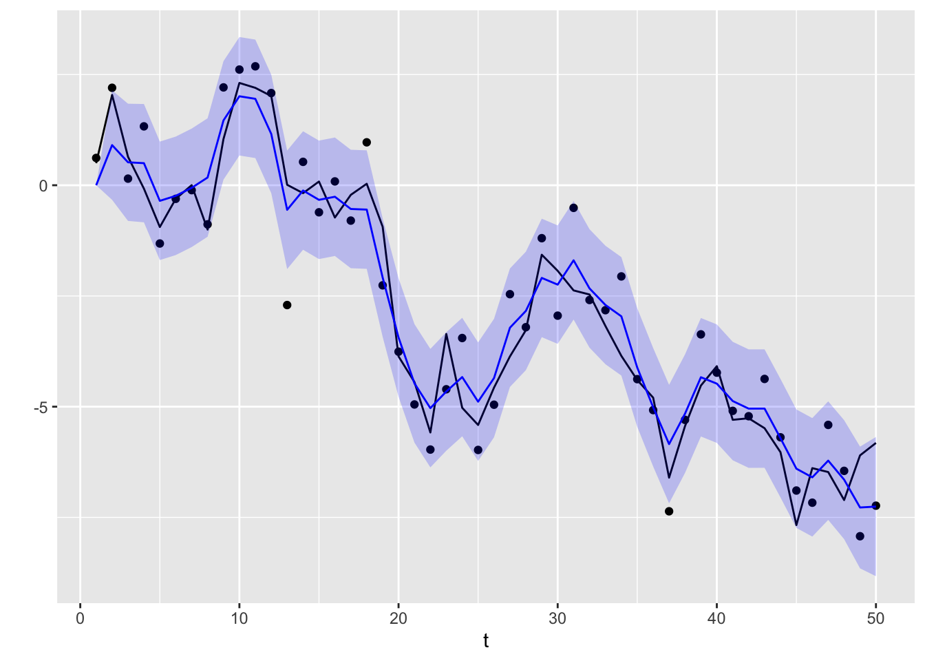
ll_dat |>ggplot(aes(x = t)) +geom_point(aes(y = yt)) +geom_line(aes(y = xt), color ="black") +geom_line(aes(y = smoothed), color ="blue") +geom_ribbon(aes(ymin = smoothed +2*sqrt(smoothed_var), ymax = smoothed -2*sqrt(smoothed_var)), fill ="blue",alpha =0.2) +ylab("")
Figure 13.7: Smoothed values for the local level model (in blue). The original values Xt are plotted as a solid black line, while the observations Yt are plotted as points. The blue region is a 95% confidence band.
Across all three plots, we see that the forecast, filtered, and smoothed values are closer than the observations \(Y_t\) to the true values \(X_t\). Furthermore, filtered values make use of more information and are thus more accurate than forecasts. Similarly, smoothed values make use of the most information, and are marginally more accurate than filtered values.
13.5.2 Global temperature
We now return to the global temperature example from Section 13.2.1. While all model parameters were known before hand in the previous example, some of the parameters have to be estimated in this example. This is done using the fitSSM() function, which is a wrapper around the optim() function from base R. It needs to be supplied with a model, as well as an update function connecting the inputs being optimized with the model parameters.
temp_dat <-tibble(ocean = gtemp_ocean /sd(gtemp_ocean), land = gtemp_land /sd(gtemp_land)) temp <- temp_dat |>as.matrix()Z <-matrix(c(1, 1, 0, 0), nrow =2) # obs matrixT <-matrix(c(1, 0, 1, 1), nrow =2) # state transitionR <-matrix(c(1, 0)) # noise embeddingQ <-matrix(NA) # state noisea1 <-matrix(c(NA, NA), nrow =2) # initial stateH <-matrix(c(NA, NA, NA, NA), nrow =2) # obs noisegtemp_model <-SSModel(temp ~SSMcustom(Z = Z, T = T, R = R, Q = Q) -1, H = H)gtemp_update <-function(pars, model) { model["Q"] <-matrix(exp(pars[1]))# L is the Cholesky factor for the noise covariance L <-matrix(c(pars[2], pars[3], 0, pars[4]), nrow =2) model["H"] <- L %*%t(L) model["a1"] <-matrix(c(pars[5], pars[6]), nrow =2) model}gtemp_fit <-fitSSM(gtemp_model, updatefn = gtemp_update, inits =c(0, 1, 0, 1, 0, 0), method ="BFGS")gtemp_out <-KFS(gtemp_fit$model, filtering ="state", smoothing ="state")
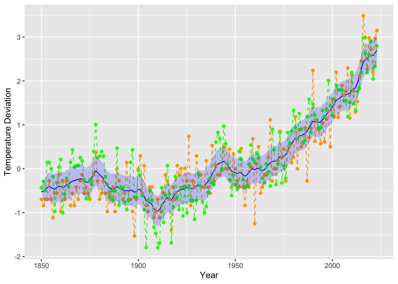
We now plot the results from fitting the model and performing filtering.
Figure 13.8: A filtered version of global temperature deviations. The green and orange lines denote the ocean and land temperatures respectively. The blue solid line denotes the filtered state values, while the blue region represents a 95% confidence region.
13.5.3 Biomarker monitoring
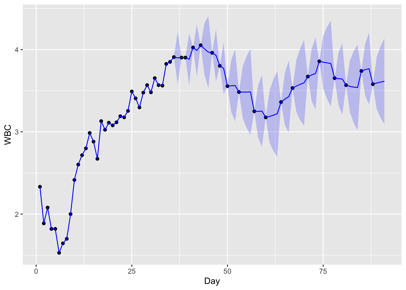
We next return to the the example from Section 13.2.3. This time, in addition to the unknown noise covariances, we also have unknown dynamics of the state. We estimate this as before using fitSSM().
Figure 13.9: Kalman filtered values for log(white blood count). The observations are plotted as points and the filtered values are plotted in blue. The blue region is a 95% confidence region.
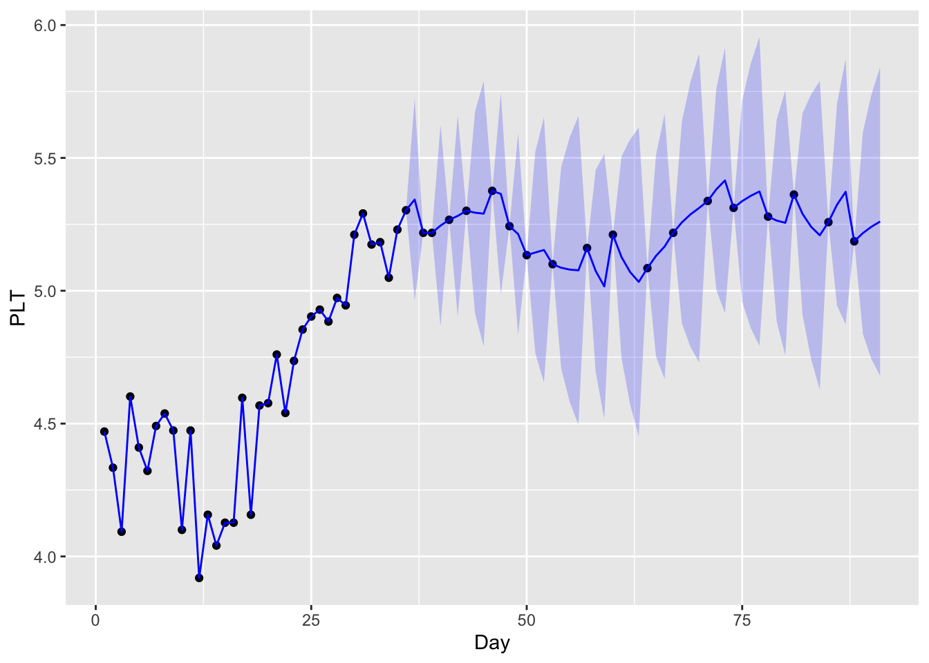
Figure 13.10: Kalman filtered values for log(platelet count). The observations are plotted as points and the filtered values are plotted in blue. The blue region is a 95% confidence region.
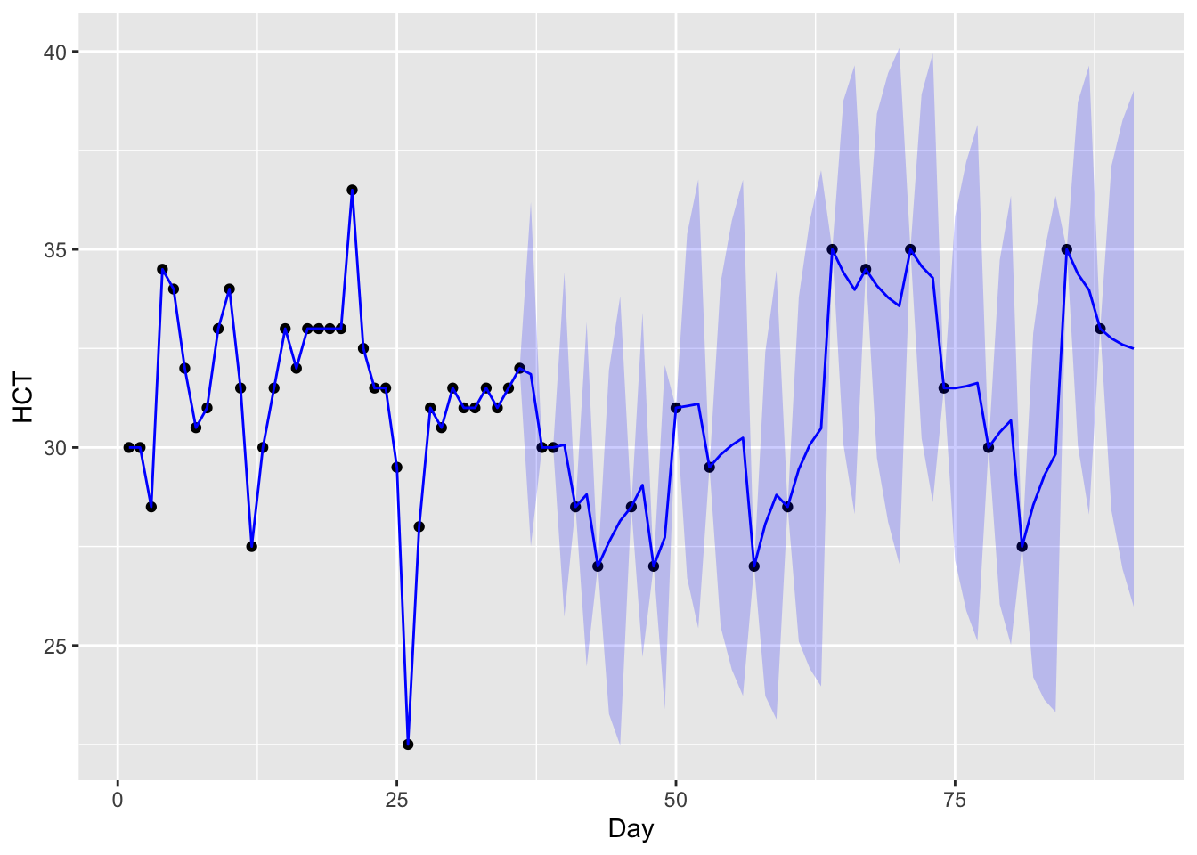
Figure 13.11: Kalman filtered values for hematrocrit. The observations are plotted as points and the filtered values are plotted in blue. The blue region is a 95% confidence region.
We may view the fitted transition matrix \(\Phi\) as follows:
To interpret this, recall that the bottom row implies that \[
X_{t,3} = -0.859 X_{t-1,1} + 1.673 X_{t-1, 2} + 0.821 X_{t-1, 3} + W_t,
\] so that the HCT value depends positively on the previous values of PLT and HCT, but negatively on the previous value of WBC.
It may be insightful to compare our results with those obtained by Shumway and Stoffer (2000) (their Example 6.9). These are somewhat different because
We have assumed zero observational noise, i.e. \(V_t = 0\).
The negative log likelihood is a non-convex function in the parameters. This means that numerical methods converge to local minima instead of a global minimum, and so different numerical optimization algorithms may lead to different solutions. Shumway and Stoffer (2000) used an algorithm called the expectation-maximization (EM) algorithm, whereas we have used BFGS.
13.6 ARIMA and ETS models
In this section, we show how ARIMA as well as ETS (exponential smoothing) models can be represented as state space models. Note that there will be some inevitable notational ambiguity, since we have used the same symbols to mean different things in Equation 13.1 and Equation 13.2 compared with in our definitions of our previous models. To reduce confusion as far as possible, we temporarily let all notation have their meaning from previous chapters. For ARIMA models, we also denote the hidden state as \(Z_t\).
13.6.1 ARIMA models
We have already shown how \(\textnormal{AR}(p)\) models can be represented as state space models. It turns out to be slightly more complicated to do this whenever a moving average component is present. We hence first show how to do this in the special case of an \(\textnormal{ARMA}(1,1)\) model.
ARMA(1, 1) model. The \(\textnormal{ARMA}(1,1)\) equation can be written as \[
Z_t = \phi Z_{t-1} + (\theta + \phi)W_{t-1},
\]\[
X_t = Z_t + W_t,
\] where \(W_t \sim WN(0,\sigma^2)\).
Proof. Using these equations, we calculate \[
\begin{split}
X_t & = Z_t + W_t \\
& = \phi Z_{t-1} + (\theta + \phi)W_{t-1} + W_t \\
& = \phi(X_{t-1} - W_{t-1}) + (\theta + \phi)W_{t-1} + W_t \\
& = \phi X_{t-1} + W_t + \theta W_{t-1},
\end{split}
\] which gives us the \(\textnormal{ARMA}(1,1)\) equation. \(\Box\)
Note that to write this as a state space model, we need to allow for noise in Equation 13.1 and Equation 13.2 to be time-correlated. This is generally the case whenever we have moving average terms in the model.
Note
Because of the time-correlated nature of the noise, we can no longer apply Propositions 13.1 and 13.2 to calculate filtered and smoothed values. Instead, we have to use a version of the Kalman filter that is adapted to this noise setting (see Property 6.5 in Shumway and Stoffer (2000)).
ARIMA model. Suppose \((X_t)\) satisfies an \(\textnormal{ARIMA}(p,d,q)\). Let \(\phi^*(z) \coloneqq \phi(z)(1-z)^d\) and denote its coefficients via \[
\phi^*(z) = 1 - \phi^*_1 z - \cdots - \phi^*_{p+d}z^{p+d}.
\] WLOG assume \(p+d \geq q\) (otherwise simply set \(\phi^*_{p+d+1} = \cdots = \phi^*_q = 0\)). Let \[
\Phi = \left[\begin{matrix}
\phi_1^* & 1 & 0 & \cdots & 0 \\
\phi_2^* & 0 & 1 & \cdots & 0 \\
\vdots & \vdots & \vdots & \ddots & \vdots \\
\phi_{p+d-1}^* & 0 & 0 & \cdots & 1 \\
\phi_{p+d}^* & 0 & 0 & \cdots & 0 \\
\end{matrix}\right],
\]\[
G =
\left[\begin{matrix}
\theta_1 + \phi_1^* \\
\vdots \\
\theta_q + \phi_q^* \\
\phi_{q+1}^* \\
\vdots \\
\phi_{p+d}^*
\end{matrix}\right].
\] Consider the \(p+d\)-dimensional state space process \((Z_t)\) defined by \[
Z_t = \Phi Z_{t-1} + G W_{t-1},
\] where \(W_t \sim WN(0,\sigma^2)\). Then \((X_t)\) can be written as \[
X_t = A Z_t + W_t,
\] where \[
A = [ 1, 0, \ldots, 0].
\]
13.6.2 Innovation state-space models
ETS methods can also be represented as state space models. Their corresponding state space models are called innovations state space models, because the same white noise process determines the randomness in both the state and observation equations.
We state here the models corresponding to simple exponential smooting and Holt linear’s method. Refer to Table 8.7 in Hyndman and Athanasopoulos (2018) for the state space models corresponding to other ETS methods.
Simple exponential smoothing. Consider the model \[
L_t = L_{t-1} + \alpha W_t,
\]\[
X_t = L_t + W_t.
\] One can check that this gives the smoothing and forecast equations for the simple exponential smoothing model (see Equation 8.3 and Equation 8.4). The likelihood of this model is proportional to the sum of squares cost function used to optimize for the parameter \(\alpha\) in SES.
Simple exponential smoothing. Consider the model \[
L_t = L_{t-1} + \alpha W_t,
\]\[
X_t = L_{t-1} + W_t.
\] One can check that this gives the smoothing and forecast equations for the simple exponential smoothing model (see Equation 8.3 and Equation 8.4).
Simple exponential smoothing with multiplicative noise. Consider the model \[
L_t = L_{t-1}(1 + \alpha W_t),
\]\[
X_t = L_{t-1}(1 + W_t).
\] This yields the same smoothing and forecasting equations as in the additive noise case. However, the likelihood will be different, leading to a different objective function for choosing \(\alpha\).
Holt’s linear method. Consider the model \[
L_t = L_{t-1} + B_{t-1} + \alpha W_t,
\]\[
B_t = B_{t-1} + \beta W_t,
\]\[
X_{t-1} = L_{t-1} + B_{t-1} + W_t.
\] This produces the smoothing and forecasting equations for Holt’s linear method (see Equation 8.5, Equation 8.6, and Equation 8.7).
Hyndman, Rob J, and George Athanasopoulos. 2018. Forecasting: Principles and Practice. OTexts.
Shumway, Robert H, and David S Stoffer. 2000. Time Series Analysis and Its Applications. Vol. 3. Springer.