9  Stationary Processes

9.1 Statistical models for time series

So far, we have worked with time series as a fixed sequence of numbers. A time series model treats the sequence of observations as a realization of a sequence random variables \(X_1,X_2,\ldots,X_n\) and specifies their joint distribution. \[ \P\lbrace X_1 \leq x_1, X_2 \leq x_2,\ldots,X_n \leq x_n\rbrace. \] Such a sequence of random variables is also called a stochastic process.¹ We will typically use upper case \((X_t)\) to denote the stochastic process, and lower case \((x_t)\) to denote a single realization. Note that in general, \(X_1,X_2,\ldots,X_n\) are not independent, nor do they even have the same marginal distribution.

Mean and autocovariance functions: We often study random variables via their moments (mean, variance, etc.). For stochastic processes, these now become functions. More precisely, the mean function of a stochastic process \((X_t)\) is defined via \[ \mu_X(t) \coloneqq \E\lbrace X_t \rbrace. \] The autocovariance function (ACVF) is defined via \[ \gamma_X(s, t) \coloneqq \Cov\lbrace X_s, X_t\rbrace. \]

In other areas of statistics, such as linear regression, one estimates the parameters of the distribution \(p\) from repeated independent measurements and then uses it to make predictions for future observations. Unfortunately, in time series problems, we typically see only a single realization of the stochastic process. Hence, in order to estimate model parameters, we have to make further assumptions on the stochastic process, such as that it satisfies some sort of regularity over time. This can be formalized using a concept called stationarity.

Strict stationarity: A strictly (or strongly) stationary stochastic process \((X_t)\) is one for which all finite-dimensional marginals of the joint distribution are shift invariant, i.e. that \[ \P\lbrace X_{t_1} \leq x_1, X_{t_2} \leq x_2,\ldots,X_{t_k} \leq x_k \rbrace = \P\lbrace X_{t_1+ h} \leq x_1, X_{t_2 + h} \leq x_2,\ldots,X_{t_k + h} \leq x_n\rbrace \] for any dimension \(k\), time indices \(t_1,t_2,\ldots, t_k\), and shift \(h\).

This definition is often too strong and diffuclt to assess. Hence, it is common to impose a milder conditions based on the first two moments.

Weak stationarity: A weakly stationary stochastic process is one for which

1. \(\mu_X(t)\) exists and is independent of \(t\), and
2. \(\gamma_X(t, t+h)\) exists for every \(t\) and \(h\) and is independent of \(t\).

Henceforth, we will use the term “stationary” to mean weakly stationary.² For such a stochastic process, we will slightly abuse notation, denoting its mean by \(\mu_X\), and its autocovariance function by \[ \gamma_X(h) = \gamma_X(t, t + h). \]

Autocorrelation function: The autocorrelation function (ACF) of a stationary process \((X_t)\) is defined as \[ \rho_X(h) = \frac{\gamma(h)}{\gamma(0)}. \] One can check that this indeed defines the correlation between \(X_t\) and \(X_{t+h}\) for any \(t\), and satisfies \(- 1 \leq \rho_X(h) \leq 1\). Note also that this function is even, i.e. \(\rho_X(-h) = \rho_X(h)\), and positive semidefinite.

Multiple processes: Given two stochastic proccesses \((X_t)\) and \((Y_t)\), their cross-covariance function is defined as \[ \gamma_{XY}(s, t) \coloneqq \Cov\lbrace X_s, Y_t\rbrace. \] If \((X_t)\) and \((Y_t)\) are each stationary, and \(\gamma_{XY}(h) \coloneqq \gamma_{XY}(t+h, t)\) is independent on \(t\), we say that they are (weakly) jointly stationary. In this case, we define their cross-correlation function (CCF) as \[ \rho_{XY}(h) = \frac{\gamma_{XY}(h)}{\sqrt{\gamma_X(0)\gamma_Y(0)}}. \] Unlike the ACF, this function is not necessarily even or positive semidefinite.

9.2 Examples

We now introduce some common examples of time series models.

9.2.1 White noise

There are three types of white noise models. We say that \((W_t)\) is a weak white noise process if it is weakly stationary, with \(\mu_X = 0\) and \[ \gamma_X(h) = \begin{cases} \sigma^2 & \text{if}~h = 0, \\ 0 & \text{otherwise}. \end{cases} \tag{9.1}\] We say that it is a strong white noise process if, in addition to the above, the sequence of random variables are independent and identically distributed. Finally, we say that it is a Gaussian white noise process if the sequence of random variables are i.i.d. Gaussian. By convention, these are all denoted using \(WN(0,\sigma^2)\).

We will soon see that many time series models are built out of transformations of a white noise process. Generally speaking, transformations of weak white noise give rise to weakly stationary processes, while transformations of strong white noise give rise to strongly stationary processes. Unless stated otherwise, however, we will assume in the rest of this book that we work with strong white noise.

9.2.2 Random walk

We say that \((X_t)\) is a random walk with drift if we have \[ X_t = \delta + X_{t-1} + W_t, \tag{9.2}\] where \((W_t) \sim WN(0,\sigma^2)\). \(\delta\) is called the drift of the walk, and if \(\delta = 0\), \((X_t)\) is called a simple random walk. Note that a random walk is not stationary, even when there is no drift. Indeed, assuming the initial condition \(X_0 = 0\) and rewriting Equation 9.2 as \[ X_t = t\delta + \sum_{j=1}^t W_j, \] we easily compute \(\mu_X(t) = \delta t\) and \[ \gamma_X(s, t) = \sigma^2\min\lbrace s, t\rbrace. \]

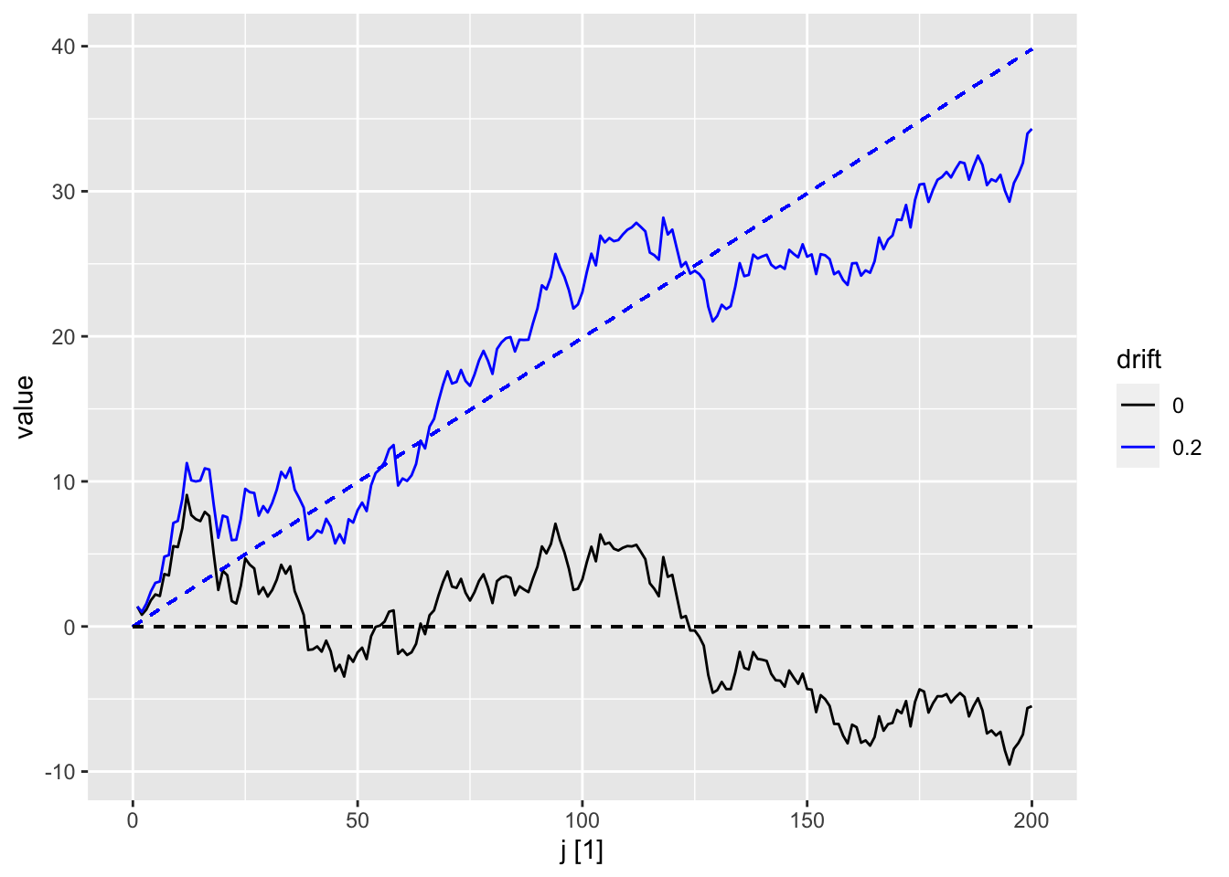
Sample trajectories for two random walks with different drift values are shown in the following plot.

set.seed(42)

rw_ts <- tibble(
    j = 1:200,
    wn = rnorm(200),
    rw0 = cumsum(wn),
    rw1 = rw0 + 0.2 * (j - 1)
    ) |> as_tsibble(index = j)

rw_ts |>
    pivot_longer(cols = c("rw0", "rw1"),
                 values_to = "value",
                 names_to = "drift") |>
    autoplot(value) + 
    geom_segment(aes(x = 0, y = 0, xend = 200, yend = 199 * 0.2),
                 linetype = "dashed", color = "blue") +
    geom_segment(aes(x = 0, y = 0, xend = 200, yend = 0),
                 linetype = "dashed", color = "black") + 
    scale_color_discrete(labels = c("0", "0.2"), type = c("black", "blue"))

Figure 9.1: Trajectories for a simple random walk (black) and a random walk with drift = 0.2. The dotted lines show have slope equal to 0 and 0.2 respectively and reflect the mean function for both processes.

Recall that the random walk model gives rise to the naive and drift forecasting methods (Section 7.2). As such, the implicit assumption we make when using these methods is that the time series looks like one of these trajectories.

9.2.3 Signal plus noise

A signal in noise model is of the form \[ X_t = f_t + W_t, \] where \((f_t)\) is a deterministic sequence of values and \((W_t) \sim WN(0,\sigma^2)\). Usually, \(f_t\) has a simple functional form, such as a sinusoidal function. Here, the first term is usually regarded as a signal, while the second term is regarded as measurement noise to be removed. This can be done using smoothing techniques, or, if the functional form is known in advance, via simple linear regression onto a convenient function basis. Note that this process is not stationary unless \(f_t\) is constant.

• When \(f_t = \beta_0 + \beta_1 t\), this time series model gives rise to the linear trend method.
• We can also view \(f_t\) as a function of other known, concurrent time series which are treated as deterministic, i.e. \(f_t = f(Z_{1t},Z_{2t},\ldots,Z_{rt})\).

9.2.4 Linear process

A linear process is defined as a convolution between a white noise process and a sequence of coefficients. Specifically, it is given by \[ X_t = \mu + \sum_{j=-\infty}^\infty \psi_j W_{t-j}, \] where \((W_t) \sim WN(0,\sigma^2)\) and \[ \sum_{j=^-\infty}^\infty |\psi_j| < \infty. \tag{9.3}\]

The mean function is constant and satisfies \(\mu_X = \mu\). We next calculate its autocovariance as follows: \[ \begin{split} \gamma_{X}(h) & = \Cov\left\lbrace \sum_{i=-\infty}^\infty \psi_i W_{t + h-i}, \sum_{j=-\infty}^\infty \psi_j W_{t-j} \right\rbrace \\ & = \sum_{i=-\infty}^\infty\sum_{j=-\infty}^\infty \psi_i \psi_j \Cov\lbrace W_{t+h-i}, W_{t-j}\rbrace \\ & = \sum_{i=-\infty}^\infty\sum_{j=-\infty}^\infty \psi_i \psi_j \gamma_W(j-i+h) \\ & = \sigma^2\sum_{i=-\infty}^\infty \psi_i \psi_{i-h}. \end{split} \tag{9.4}\] Here, the second equality comes from the bilinear nature of covariance, while the last equality uses Equation 9.1. Finally, this value is finite because of Equation 9.3. We thus see that \((X_t)\) is stationary.

We say that a linear process is causal if \(\psi_j = 0\) for all \(j < 0\). In other words, for such a time series, the observation at time \(t\) depends only on the current and past values of the white noise process. This is an appropriate assumption when modeling real world time series.³

9.2.5 Gaussian processes

We say that \((X_t)\) is a Gaussian process if all finite dimensional projections \((X_{t_1},X_{t_2},\ldots,X_{t_k})\) have a multivariate normal distribution. The distribution of a Gaussian process is fully determined by its mean and autocovariance functions. More precisely, the density for \((X_{t_1},X_{t_2},\ldots,X_{t_k})\) is given by \[ p(x_1,x_2,\ldots,x_k) = (2\pi)^{-k/2} \det(\Gamma)^{-1/2}\exp\left(-\frac{1}{2}(x_{1:k} - \mu)^T\Gamma^{-1}(x_{1:k} - \mu)\right), \] where \(x_{1:k} = (x_1,x_2,\ldots,x_k)\), \(\mu = (\mu_X(t_1),\ldots,\mu_X(t_k))\), and \(\Gamma_{ij} = \gamma_X(t_i, t_j)\).

If \((X_t)\) is weakly stationary, then \(\mu\) is a constant vector and the entries of \(\Gamma\) depend only on the differences \(|t_i - t_j|\). In particular it is strongly stationary.

9.3 Moment estimation

In Chapter 6, we learnt about sample versions of the mean, autocovariance function, and autocorrelation function. It turns out that when the time series is drawn from a stationary linear process, all three are consistent and asymptotically normal estimators of their population counterparts, as the length \(n\) of the time series converges to infinity. As we will soon see, this allows us to perform hypothesis testing in various scenarios.

Theorem 9.1 (Mean). If \((X_t)\) is a stationary linear process, then \[ \sqrt{n}\left(\bar X_n - \mu \right) \to_d N(0, V), \] where \[ V = \sum_{h = - \infty}^\infty \gamma_X(h) = \sigma^2 \left(\sum_{j=-\infty}^\infty \psi_j \right)^2. \] Furthermore, if \((X_t)\) is a linear process on Gaussian white noise, then we have \[ \bar X_n \sim N\left(\mu, \frac{1}{n}\sum_{|h| < n} \left(1 - \frac{|h|}{n}\right)\gamma_X(h)\right). \]

Proof: See Theorem A.5 of a proof of the first statement. For the second, we just need to compute the variance of \(\bar X\) as follows: \[ \begin{split} \Var\lbrace\bar X_n\rbrace & = \Var\left\lbrace \frac{1}{n}\sum_{t=1}^n X_t\right\rbrace \\ & = \frac{1}{n^2}\sum_{s,t=1}^n \Cov\lbrace X_s, X_t\rbrace \\ & = \frac{1}{n^2}\sum_{s,t=1}^n \gamma_X(t-s) \\ & = \frac{1}{n}\sum_{h=-n}^n \left(1 - \frac{|h|}{n} \right)\gamma_X(h). \end{split} \]

Theorem 9.2 (ACF). If \((X_t)\) is a stationary linear process based on white noise with finite 4th moments⁴, then for any fixed \(k\), \[ \sqrt{n}\left(\hat\rho_{1:k} - \rho_{1:k}\right) \to_d N(0, V), \] where \(\rho_{1:k} = (\rho_X(1),\ldots,\rho_X(k))\), \(\hat\rho_{1:k} = (\hat\rho_X(1),\ldots,\hat\rho_X(k))\), and \[ V_{ij} = \sum_{u=1}^\infty \left(\rho(u+i) + \rho(u-i) - 2\rho(i)\rho(u)\right)\left(\rho(u+j) + \rho(u-j) - 2\rho(j)\rho(u)\right). \] In particular, if \((X_t)\) is white noise, then \[ \sqrt{n}\rho_{1:k} \to_d N(0,I). \]

Proof: See Theorem A.7 in Shumway and Stoffer (2000).

Note that the ACVF and the CCF both have similar limiting behavior. See Theorem A.6 and Theorem A.8 in Shumway and Stoffer (2000) for more details.

9.4 Applying models to data

Time series models are useful for several different time series tasks, such as forecasting, smoothing, regression, simulation, and anomaly detection. Here, we focus on their use in forecasting.

The simple forecasting methods as well as exponential smoothing methods allow us to exploit trend and seasonality patterns for forecasting. However, they are not able to make use of short-term cycles or, more generally, any patterns in the remainder component of a time series decomposition. On the other hand, unless the remainder component comprises white noise, time-based correlations exist, and these can be used to improve forecasts. This is addressed by the Box-Jenkins method, which we now discuss.

The Box-Jenkins method, named after George Box and Gwilym Jenkins, was formulated in their textbook Box et al. (2015).⁵ It roughly involves the following steps:

Step 1: Transform the time series \((X_t)\) to make it stationary using time series decomposition, differencing, and/or Box-Cox transformations.

Step 2: Identify the correct model to fit to the transformed time series \((Y_t)\).

Step 3: Fit the model and estimate the model coefficients.

Step 4: Check whether the residuals from Step 3 are white noise. If so, we are done. If not, return to Step 2.

Step 5: To forecast for \((X_t)\), first forecast for the transformed time series, then back transform the forecasts.

The Box-Jenkins method is certainly not the only approach to time series modeling and forecasting. Nonetheless, it is quite influential and remains very useful. It underpins our interest in modeling stationary time series.

Typically, the model fit in Step 2 is an AutoRegressive Moving Average (ARMA) model, which we will learn about in Chapter 10. We next discuss Step 1 and Step 4 in more detail in the next two sections.

9.5 Two types of non-stationarity

There are two common types of non-stationarity, each of which are best handled using different techniques.

Trend stationarity: We say that \((X_t)\) is trend stationary if \[ X_t = f_t + Y_t, \tag{9.5}\] where \((f_t)\) is a deterministic sequence and \((Y_t)\) is a stationary process. Note that, the terminology notwithstanding, \(f_t\) may include trend, seasonality, as well as long-term cycles. In this case, one can try to estimate \(f_t\) and subtract it from \(X_t\) in order to obtain a stationary sequence. This is of course just time series decomposition and one can use the techniques learned in Chapter 5 to do this. If \(f_t\) has a convenient functional form, or if it is a deterministic function of other known, concurrent time series, one can also perform dynamic regression.

Unit root: Unit roots require some technical jargon to define. We will defer this to Chapter 12. For now, we note that some time series cannot be made stationary via subtracting trend and seasonal components. For instance, the simple random walk falls into this category because it already has has mean and no seasonality. On the other hand, it can be made stationary by taking a difference on Equation 9.2: \[ \begin{split} Y_t & \coloneqq X_t - X_{t-1} \\ & = \delta + W_t. \end{split} \] Because taking a single first difference makes the the random walk stationary, we say that it has one unit root.

Note that taking a difference of a trend stationary process with linear trend, \(X_t = \beta_0 + \beta_1 t + Y_t\), can also make it stationary. Indeed, we have \[ X_t - X_{t-1} = \beta_1 + Y_t - Y_{t-1}, \] and the first difference of a stationary sequence remains stationary (check this.) More generally, when \(f_t\) in Equation 9.5 is a degree \(k\) polynomial, it can be made stationary by taking differences \(k\) times. However, it is not recommended to use differencing on trend stationary time series. This is because taking differences leads to instability when inverting the differencing to forecast for the original time series (Step 5 of Box-Jenkins). Recall our interpretation of differencing as discrete differentiation, this phenomenon is analogous to how small changes in derivatives \(g'\), \(g''\), etc. can lead to large changes in the behavior of the original function \(g\).

There are various tests for stationarity and for the presence of unit roots, such as the Durbin-Watson test and the KPSS test. We will discuss them in further detail in Chapter 12.

Note

These are not the only types of non-stationarity. Consider for instance the case where we have a multiplicative time series decomposition.

9.6 Testing for white noise

If the residuals in Step 3 are not white noise, then we could in principle use the remaining autocorrelations to improve our forecast model. Hence, it is important to know how to test whether the residuals are indeed white noise.

9.6.1 Three tests

There are several ways of testing whether \((X_t)\) is a white noise sequence. These tests are mostly based on the asymptotic normality of the ACF. Note further that while the null hypothesis is that \((X_t)\) is white noise, the alternative is not clearly defined.⁶

Visual “test”: We can inspect the ACF plot. Note that in an ACF plot generated using ACF() |> autoplot(), the dotted blue horizontal lines are positioned at \(\pm 1.96/\sqrt{n}\). Under the null hypothesis that \((X_t)\) is white noise, then by the second theorem in Section 9.3, the spikes should be approximately i.i.d. Gaussian, with variance \(1/n\), which means that each spike should not exceed these lines with 95% probability.

Box-Pierce test: Define the Box-Pierce test statistic: \[ Q_{BP} \coloneqq n\sum_{j=1}^h \hat\rho_X(j)^2. \] By the continuous mapping theorem, we have \(Q_{BP} \to_d \chi^2_{h}\) under the null hypothesis. In other words, in converges in distribution to a chi-squared distribution with \(h\) degrees of freedom. The Box-Pierce test thus rejects \(H_0\) when \(Q_{BP}\) is larger than the \(1-\alpha\) quantile of \(\chi^2_h\). Alternatively, if we let \(F\) denote the quantile function of \(\chi^2_h\), we obtain a p-value via computing \(1 - F(Q_{BP})\).

Ljung-Box test Define the Ljung-Box test statistic: \[ Q_{LB} \coloneqq n(n+2)\sum_{j=1}^h \frac{\hat\rho_X(j)^2}{n-j} \tag{9.6}\] Asymptotically, we also have \(Q_{LB} \to_d \chi^2_{h}\) under the null hypothesis, and one can use \(Q_{LB}\) in exactly the same would you would use \(Q_{BP}\). On the other hand, it has been found that the distribution of \(Q_{LB}\) is closer to \(\chi^2_{h}\) than that of \(Q_{BP}\) in finite samples. Hence, the Ljung-Box test is usually preferred to the Box-Pierce test.

Note that both the Box-Pierce test and the Ljung-Box test come with a tuning parameter: \(h\). Hence, each actually comprises a family of hypothesis tests. There does not seem to be an established best practice on how to pick \(h\). Hyndman and Athanasopoulos (2018) recommend setting \(h = \min\lbrace 10, n/5\rbrace\) for non-seasonal data, and \(h = \min\lbrace 2p, n/5\rbrace\) for seasonal data, where \(p\) is the period of the seasonality. Here, the logic is that \(h\) should be large enough so that it can include any troublesome ACF values, but not too large as in that case, the test statistic may be quite different from the reference \(\chi^2_h\) distribution.⁷

Note also that if the time series to be tested, \((X_t)\), comprises the residuals of a fitted model with \(r\) parameters, then \(Q_{LB}\) and \(Q_{BP}\) actually converge to \(\chi^2_{h-r}\), which tends to have smaller values. Hence, we can obtain a more powerful test by comparing their values with the quantiles of this reference distribution.

There are also a number of other tests that can be used, such as the Breusch-Godfrey test or the difference-sign test. We refer the interested reader to Chapter 1.6 of Brockwell and Davis (1991).

9.6.2 Example 1: Apple stock

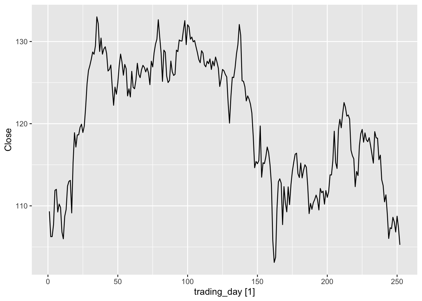
We now try to model Apple daily closing stock prices in 2015. We first create and plot the data as follows:

apple_2015 <- gafa_stock |> 
    filter(Symbol == "AAPL") |> 
    filter(year(Date) == 2015) |> 
1    mutate(trading_day = row_number()) |>
    as_tsibble(index = trading_day, regular = TRUE)

apple_2015 |>
    autoplot(Close)

1

We create a new index column because the stock market is closed on weekends and holidays.

Figure 9.2: Apple daily closing stock price in 2015.

From the above plot, we see that the stock price seems to be similar to a random walk, so we try to model it using the naive method. We then apply the “visual” test to the residuals \(x_t - x_{t-1}\).

apple_fit <- apple_2015 |> 
    model(Naive = NAIVE(Close))
    
apple_fit |> 
    gg_tsresiduals()

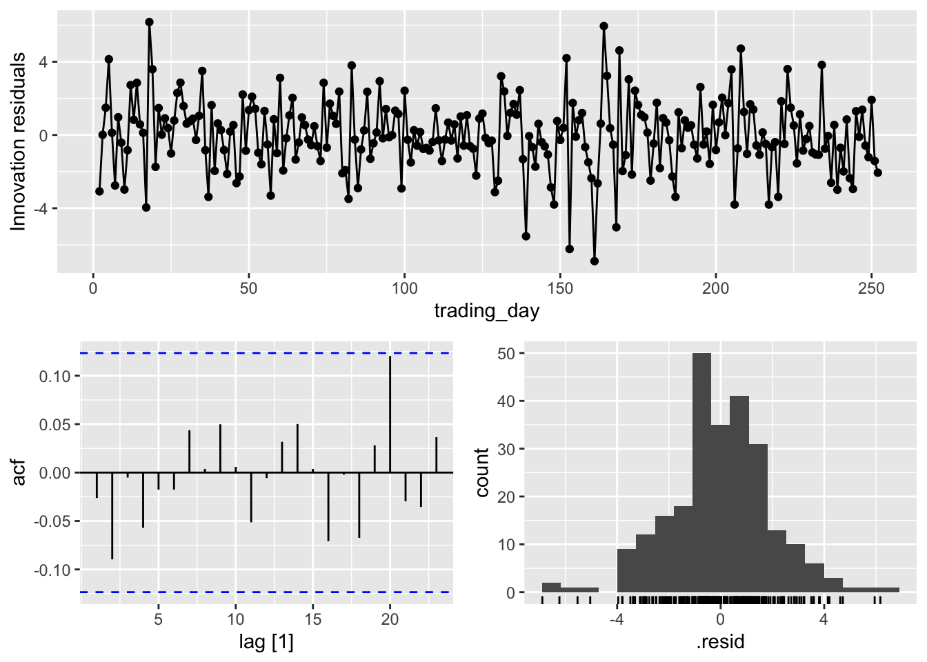
Figure 9.3: Residual diagnostics for the naive method applied to Apple daily closing stock price in 2015.

Here, the function gg_tsresiduals() has automatically generated three plots for the residuals of the model:

1. (Top) A time plot
2. (Bottom left) An ACF plot
3. (Bottom right) A histogram

Outside of some outlier values around day 150, the rest of the values seem to be drawn from an i.i.d. Gaussian distribution. We can check this further using the Ljung-Box test. Below, we first create a table containing the residuals using the function augment().

apple_fit |>
    augment()

# A tsibble: 252 x 7 [1]
# Key:       Symbol, .model [1]
   Symbol .model trading_day Close .fitted  .resid  .innov
   <chr>  <chr>        <int> <dbl>   <dbl>   <dbl>   <dbl>
 1 AAPL   Naive            1  109.     NA  NA      NA     
 2 AAPL   Naive            2  106.    109. -3.08   -3.08  
 3 AAPL   Naive            3  106.    106.  0.0100  0.0100
 4 AAPL   Naive            4  108.    106.  1.49    1.49  
 5 AAPL   Naive            5  112.    108.  4.14    4.14  
 6 AAPL   Naive            6  112.    112.  0.120   0.120 
 7 AAPL   Naive            7  109.    112. -2.76   -2.76  
 8 AAPL   Naive            8  110.    109.  0.970   0.970 
 9 AAPL   Naive            9  110.    110. -0.420  -0.420 
10 AAPL   Naive           10  107.    110. -2.98   -2.98  
# ℹ 242 more rows

Note that there are two types of residuals in this table. The column labeled .resid comprises the residuals \(x_t - \hat x_{t|t-1}\). The column labeled .innov comprises the innovation residuals. These are the residuals of the transformed time series if a transformation was performed on the time series prior to forecasting, and are equal to the regular residuals if no transformation was performed.

We now perform Ljung-Box on the innovation residuals.

apple_fit |>
    augment() |>
    features(.innov, ljung_box, lag = 10)

# A tibble: 1 × 4
  Symbol .model lb_stat lb_pvalue
  <chr>  <chr>    <dbl>     <dbl>
1 AAPL   Naive     4.39     0.928

Here, we see that the p-value is much larger than 0.05, so we do not reject the null hypothesis that the residuals are white noise. In other words, the random walk model / naive method seems to have a good fit to the data.

9.6.3 Example 2: Tourist arrivals to Australia

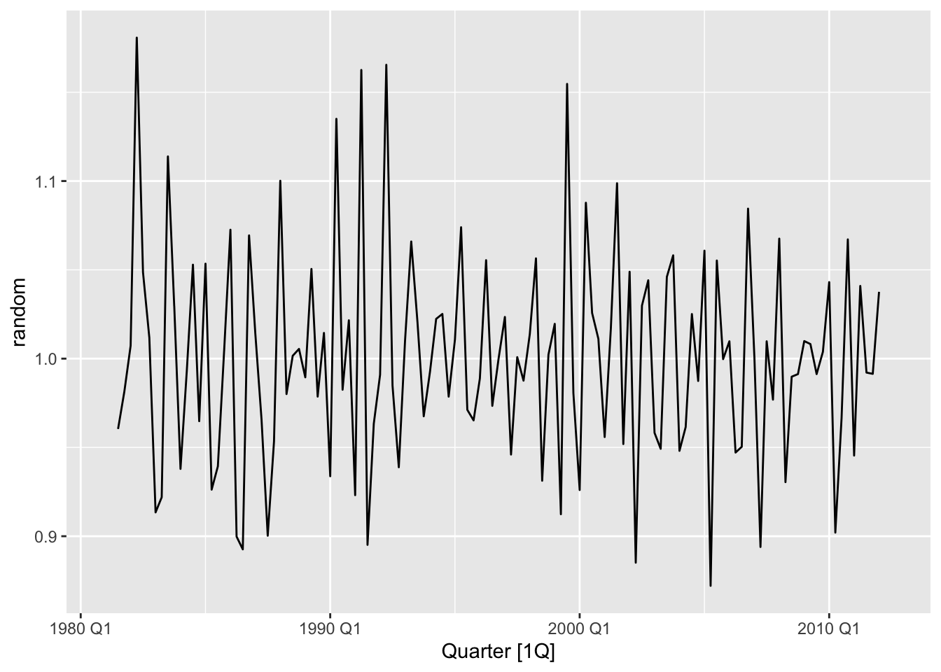
Recall our use of classical decomposition to model tourist arrivals to Australia from the UK (Section 5.4). Let us now check whether the remainder component of the decomposition are white noise. We first generate this time series as follows.

arrivals_ausjap_remainder <- aus_arrivals |>
    filter(Origin == "UK") |>
    model(
        classical_decomposition(Arrivals, type = "multiplicative")
        ) |>
    components() |>
    select(Quarter, random)

Next, we make time and ACF plots.

Time plot

arrivals_ausjap_remainder |>
    autoplot(random)

Figure 9.4: Remainder component of a classical decomposition of tourist arrivals to Australia from the UK.

ACF plot

arrivals_ausjap_remainder |>
    ACF(random) |>
    autoplot()

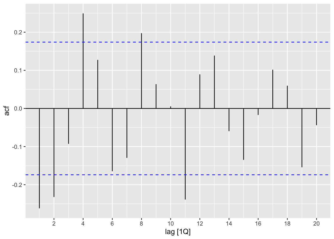
Figure 9.5: ACF of remainder component of a classical decomposition of tourist arrivals to Australia from the UK.

From the ACF plot, we see that there are a number of spikes that lie outside of the confidence band for white noise. Finally, we compute the p-value for the Ljung-Box test at lag \(h = 4 * 2 = 8\). This is very small, confirming our suspicions that the remainder component is significantly different from white noise.

arrivals_ausjap_remainder |>
    features(random, ljung_box, lag = 8)

# A tibble: 1 × 2
  lb_stat  lb_pvalue
    <dbl>      <dbl>
1    37.8 0.00000837

Box, George EP, Gwilym M Jenkins, Gregory C Reinsel, and Greta M Ljung. 2015. Time Series Analysis: Forecasting and Control. John Wiley & Sons.

Brockwell, Peter J, and Richard A Davis. 1991. Time Series: Theory and Methods. Springer science & business media.

Hyndman, Rob J, and George Athanasopoulos. 2018. Forecasting: Principles and Practice. OTexts.

Shumway, Robert H, and David S Stoffer. 2000. Time Series Analysis and Its Applications. Vol. 3. Springer.

---

1. In the setting of time series models, we will use the terms “stochastic process” and “time series” interchangeably.

2. As a slight variant of this, we call a stochastic process covariance stationary if 2 holds, but with no requirement on the mean function.

3. Indeed, linear processes have surprising generality. The Wold decomposition theorem states that every covariance-stationary time series can be written as the sum of a linear process as well as a predictable sequence.

4. \((W_t)\) has finite 4th moments if \(\E W_t^4 < \infty\) for all \(t\).

5. The book was first published in 1970 but has since been reprinted.

6. Such a hypothesis test is sometimes called a portmanteau test, although the there seems to be some confusion about the meaning of the term in the literature.

7. See https://robjhyndman.com/hyndsight/ljung-box-test/ for a more extended discussion.