7  Introduction to Forecasting

\[ \newcommand{\data}[1][n]{\mathcal{D}_{#1}} \newcommand{\E}{\mathbb{E}} \]

One of the primary goals of time series analysis is forecasting. By analyzing historical data patterns, we can make predictions about future values. For instance, investment companies make profits based on their ability to forecast stock prices and volatility. Forecasting weather patterns allows us to plan our daily activities more effectively. During the Covid pandemic, it was important for governments to forecast Covid case counts in order to allocate medical resources and to make policy decisions such as whether or not to trigger social distancing measures. In this chapter, we create a formal framework for forecasting, discuss various strategies for forecasting, introduce prediction intervals, and talk about how to evaluate forecast accuracy.

7.1 The target of a forecast

Forecasting is about predicting future values for a time series given its past values and possibly those of covariates and other concurrent predictor time series. More formally, in the simplest setting, we have an observed time series \[ x_1,x_2,\ldots,x_n \tag{7.1}\] and would like to predict unobserved future values \(x_{n+1}, x_{n+2}, \ldots\) For any \(h\), an estimate of \(x_{n+h}\) given Equation 7.1 is called a forecast and is denoted as \(\hat x_{n+h|n}\). Here, \(h\) is called the forecast horizon. The subscript is indicative of both the forecast horizon as well as the data used to generate the forecast.

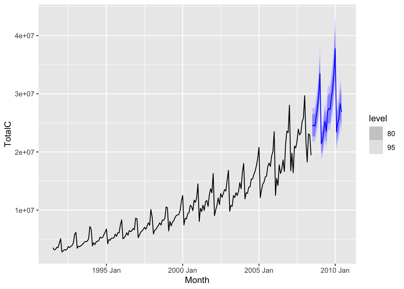
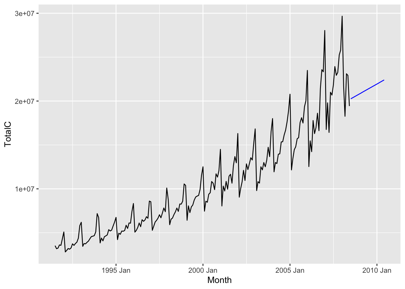
Visually, we can think of forecasting as generating something like the following plot.

Figure 7.1: Forecasting sales numbers for antidiabetic drugs in Australia.

Here, we used the time series measuring sales of antidiabetic drugs in Australia between 1991 and 2008 to forecast sales of the same genre of drugs between 2008 and 2010. The black line indicates observed historical values, while the blue line represents the forecast. The blue region around the blue line represents a “confidence region” for the forecast.

Of course, producing a forecast requires a choice of model or method. We present a few simple methods in the next section.

7.2 Simple forecasting methods

7.2.1 Mean method

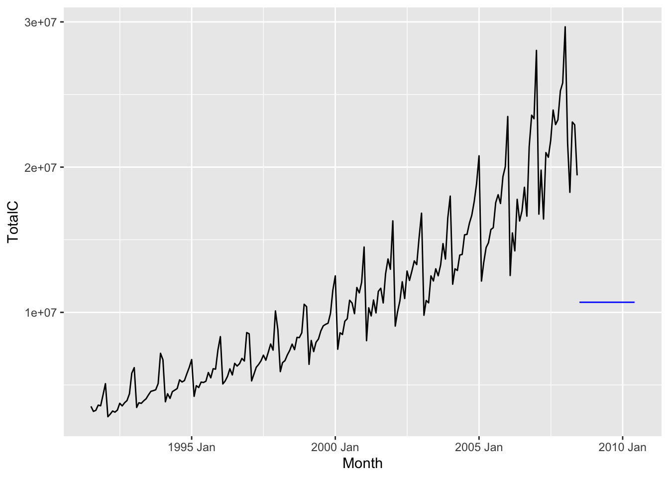
For any forecast horizon \(h\), we define the forecast as the mean of the observed historical values, i.e. \[ \hat x_{n + h|n} := \frac{1}{n}\sum_{t=1}^n x_t. \] The result for the antidiabetic drug sales dataset is shown below.

Figure 7.2: Forecasting sales numbers for antidiabetic drugs in Australia using the mean method.

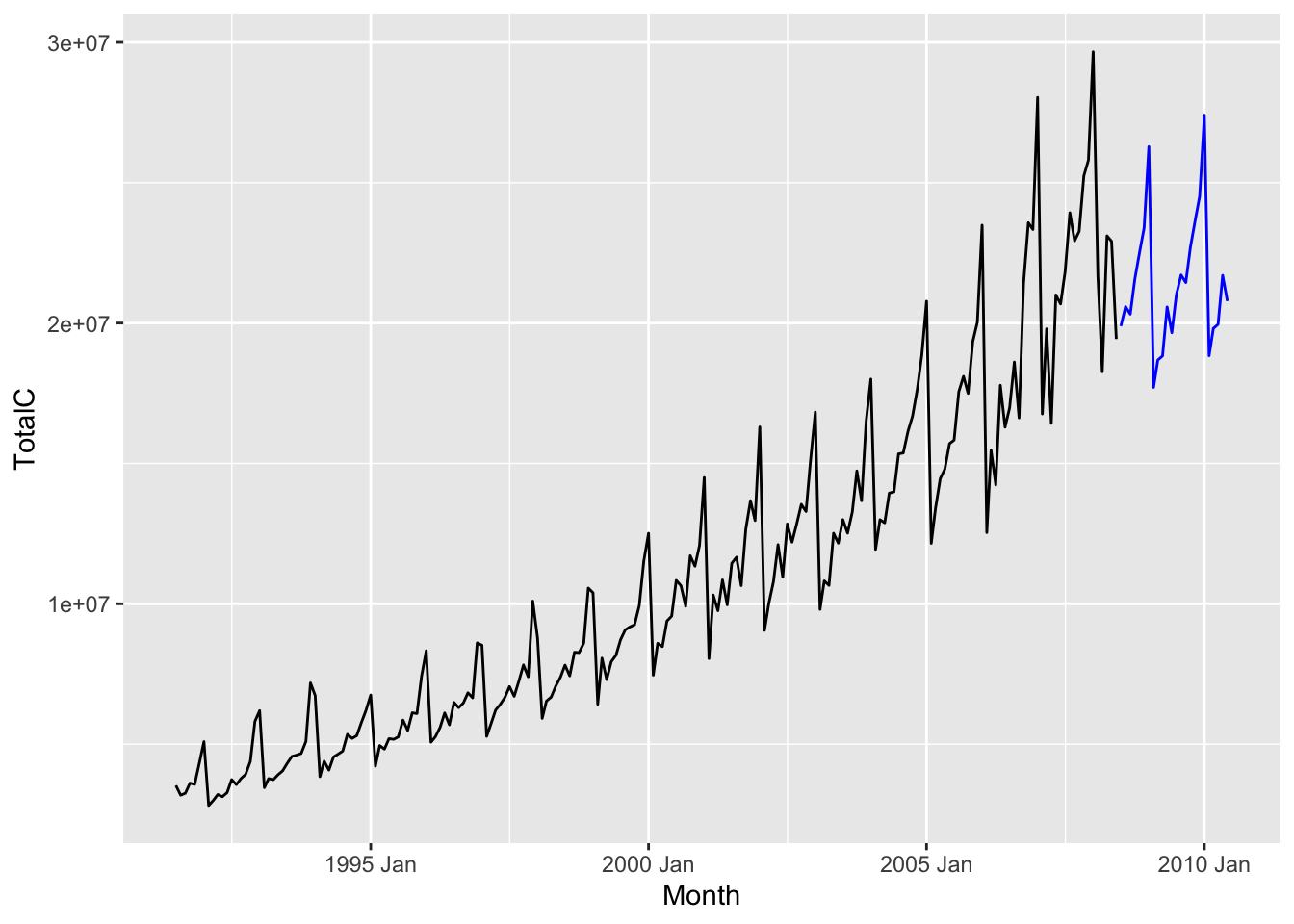
7.2.2 Naive method

For any forecast horizon \(h\), we define the forecast as the value of the most recent observation, i.e. \[ \hat x_{n + h|n} := x_n. \] The result for the antidiabetic drug sales dataset is shown below.

Figure 7.3: Forecasting sales numbers for antidiabetic drugs in Australia using the naive method.

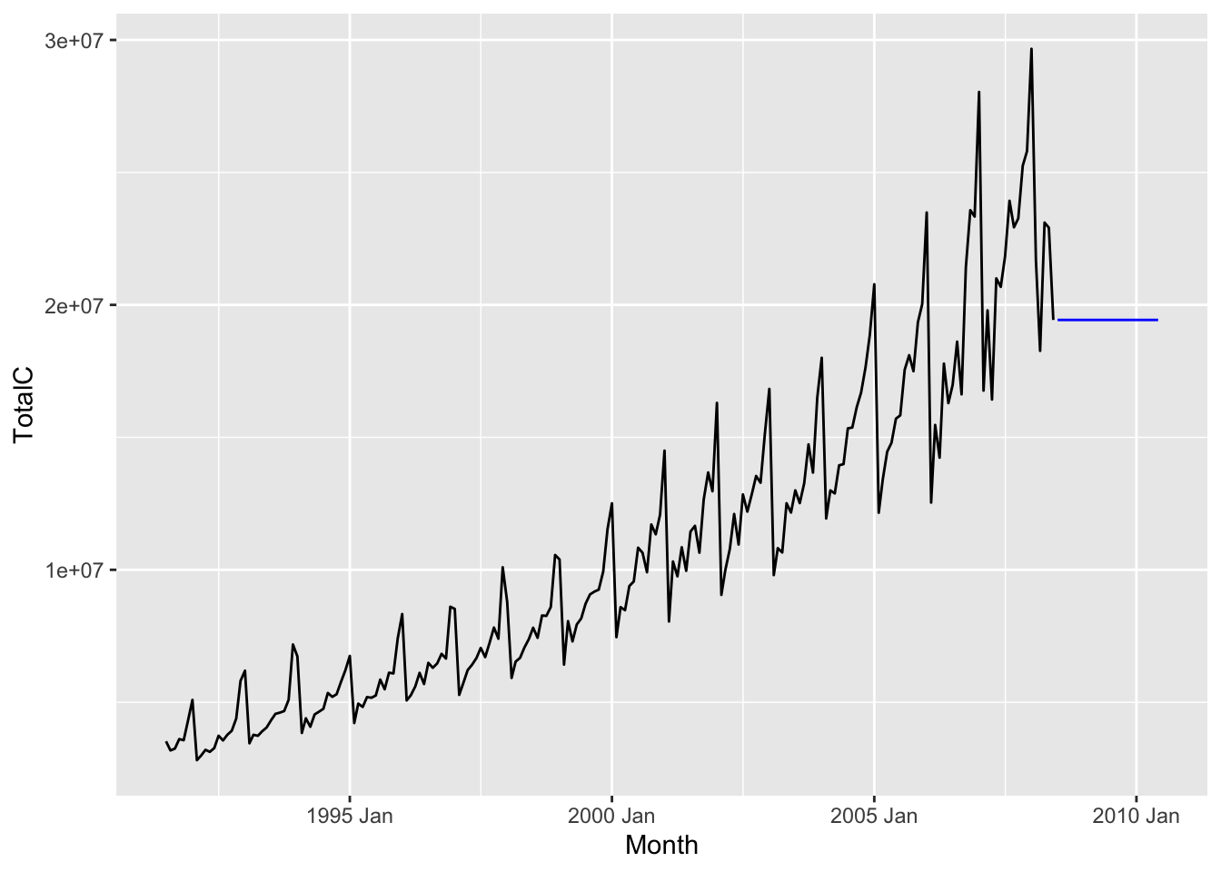
The naive method is especially useful when the time series is a martingale, i.e. similar to a random walk. This is a good model for stock prices over the short term, but clearly not a good model for the antidiabetic drug sales dataset.

7.2.3 Seasonal naive method

For any forecast horizon \(h\), we define the forecast to be equal to the most recent observation from the same season, i.e. \[ \hat x_{n + h|n} := x_{n - p + (h~\text{mod}~p)}, \] where \(h~\text{mod}~p\) refers to the integer remainder of \(h\) after dividing by \(p\). The result for the antidiabetic drug sales dataset is shown below. Since the seasonality is yearly, the forecast for January 2010 is the value of the sales in January 2008.

Figure 7.4: Forecasting sales numbers for antidiabetic drugs in Australia using the seasonal naive method.

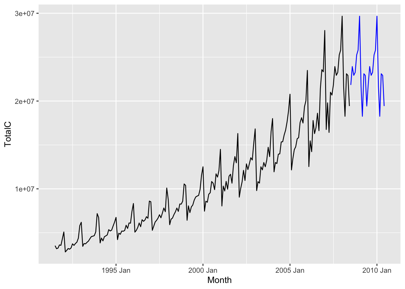
The seasonal naive method is useful when the time series is dominated by seasonality.

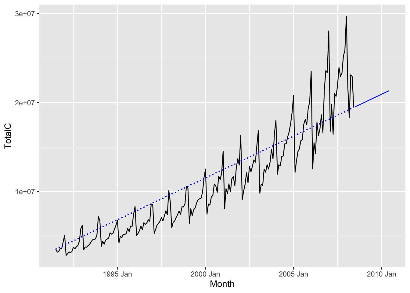
7.2.4 Linear trend method

Just as in univariate linear regression, the linear trend method fits a best fit line to all the observed time series values, and uses it to extrapolate to future values. In other words, we fit the model \[ x_t = \beta_0 + \beta_1 t + \epsilon, \] where \(t\) is the time index variable. The forecast for any time horizon \(h\) is then \[ \hat x_{n + h | n } = \hat \beta_0 + \hat \beta_1 (n+h). \]

Figure 7.5: Forecasting sales numbers for antidiabetic drugs in Australia using the linear trend method.

The linear trend method is useful when the time series is dominated by a trend that is linear.

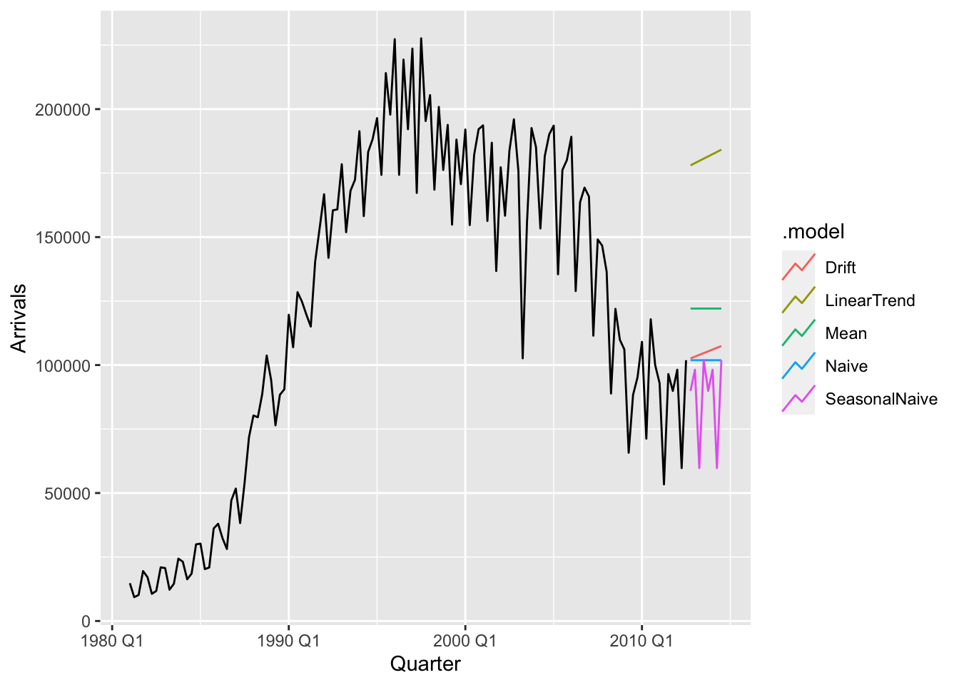
7.3 Forecasting using fable

The fable package contains a wide array of modeling choices and a simple and organized interface for fitting models, making forecasts, and evaluating models. This section gives an overview of the tools provided and how to use them. The following code snippet fits all the models described above to the aus_arrivals dataset:

arrivals_fit <- aus_arrivals |> 
    model(
        Mean = MEAN(Arrivals),
        Naive = NAIVE(Arrivals),
        SeasonalNaive = SNAIVE(Arrivals),
        LinearTrend = TSLM(Arrivals ~ trend())
        )
arrivals_fit

# A mable: 4 x 5
# Key:     Origin [4]
  Origin    Mean   Naive SeasonalNaive LinearTrend
  <chr>  <model> <model>       <model>     <model>
1 Japan   <MEAN> <NAIVE>      <SNAIVE>      <TSLM>
2 NZ      <MEAN> <NAIVE>      <SNAIVE>      <TSLM>
3 UK      <MEAN> <NAIVE>      <SNAIVE>      <TSLM>
4 US      <MEAN> <NAIVE>      <SNAIVE>      <TSLM>

Note that the object returned by model() is a mable (model table). It contains a column for every method specified and a row for every time series in the tsibble supplied to model(). Each entry comprises a fitted model using the corresponding method and for the corresponding time series.

To generate forecasts, we use the function forecast(), as in the follow snippet:

arrivals_fc <- arrivals_fit |> forecast(h = 8)
arrivals_fc

# A fable: 128 x 5 [1Q]
# Key:     Origin, .model [16]
   Origin .model Quarter           Arrivals   .mean
   <chr>  <chr>    <qtr>             <dist>   <dbl>
 1 Japan  Mean   2012 Q4 N(122080, 4.2e+09) 122080.
 2 Japan  Mean   2013 Q1 N(122080, 4.2e+09) 122080.
 3 Japan  Mean   2013 Q2 N(122080, 4.2e+09) 122080.
 4 Japan  Mean   2013 Q3 N(122080, 4.2e+09) 122080.
 5 Japan  Mean   2013 Q4 N(122080, 4.2e+09) 122080.
 6 Japan  Mean   2014 Q1 N(122080, 4.2e+09) 122080.
 7 Japan  Mean   2014 Q2 N(122080, 4.2e+09) 122080.
 8 Japan  Mean   2014 Q3 N(122080, 4.2e+09) 122080.
 9 Japan  Naive  2012 Q4  N(1e+05, 6.9e+08) 101900 
10 Japan  Naive  2013 Q1  N(1e+05, 1.4e+09) 101900 
# ℹ 118 more rows

Here, the argument \(h = 8\) specifies the forecast horizon to be 12 time units. The code returns a fable (forecast table), in which each row is a forecast by a given model (.model), for a particular time series (Origin), at a particular time point (Quarter). Since we have set \(h = 8\), we have forecasts for the 8 quarters after the last observation, which was 2012 Q3. Note also that the forecast comprises not just a single value (.mean), but also an entire distribution (Arrivals). This distribution is used to generate the confidence region shown in Figure 7.1. We will discuss this more in Section 7.9.

Finally, to plot the forecasts as in Figure 7.1, we apply autoplot() to the fable.

arrivals_fc |>
1    filter(Origin == "Japan") |>
2    autoplot(aus_arrivals,
3             level = NULL)

1

We filter arrivals_fc to only show the forecast for arrivals from Japan.

2

As a second argument to autoplot(), we also supply the original values of the time series so that these can also be plotted.

3

We set the level to be NULL so as to hide the confidence region.

7.4 Forecasting with decomposition

While the seasonal naive method is useful for forecasting time series with seasonality and the linear trend method is useful for forecasting time series with linear trend, real world time series often contain multiple patterns. We would like to simultaneously use both patterns for forecasting. One way to do so is to make use of time series decompositions, which we learnt about in Chapter 5.

We first decompose our time series into seasonal and seasonally-adjusted components: \[ x_t = \hat S_t + \hat A_t. \] Note that the seasonally adjusted component is simply the sum of the trend-cycle and remainder components. Then, we can forecast for \(\hat S_t\) and \(\hat A_t\) separately, before adding these values together to get a forecast for \(x_t\). In other words, the forecast for any forecast horizon \(h\) is given by \[ \hat x_{n+h|n} := \hat S_{n+h|n} + \hat A_{n+h|n}. \]

fable provides a convenient and concise interface for implementing such a modeling approach.

diabetes |> 
1    model(StlModel = decomposition_model(
2        STL(TotalC),
3        TSLM(season_adjust ~ trend()),
4        SNAIVE(season_year))
     ) |>
    forecast(h = 24) |>
    autoplot(diabetes, level = NULL)

1

We use the function decomposition_model() to specify that we would like to perform a decomposition and then fit individual models to separate components.

2

The first argument to decomposition_model() is the method for the time series decomposition. Here, we have chosen to perform an STL decomposition.

3

Here, we specify using the linear trend method to model the seasonally adjusted component, identified as seasonal_adjust. ¹

4

Finally, we specify using the seasonal naive method to model the seasonal component identified as season_year. If this line is omitted from the snippet, decomposition_model() will automatically fit a seasonal naive method to this component. We include it here for completeness.

Figure 7.6: Forecasting sales numbers for antidiabetic drugs in Australia using a decomposition method.

Compared to Figure 7.4, we see that the forecasts from the decomposition forecasting model is less sensitive to the shape of the most recent repeating unit (because of the STL smoothing), and has an upward trend, both of which are arguably desirable properties in this scenario.

7.5 Transformations

We have seen in Chapter 4 how to stabilize variance using Box-Cox transformations. Such transformations can be applied to a time series before forecasting, in order to improve forecast accuracy. After forecasting the transformed time series, the forecasts have to be back-transformed to obtain forecasts for the original time series. Thankfully, fable can do this automatically for us.

diabetes |> 
    model(StlModel = decomposition_model(
1        STL(log(TotalC)),
        TSLM(season_adjust ~ trend()),
        SNAIVE(season_year))
     ) |>
    forecast(h = 24) |>
    autoplot(diabetes, level = NULL)

1

We apply the log transform to the column name provided to the modeling function (in this case it is STL).

Figure 7.7: Forecasting sales numbers for antidiabetic drugs in Australia using a log transform and a decomposition method.

Compared to Figure 7.6, we see that the modeled trend is now exponentially increasing, and so are the fluctuations.

7.6 Statistical models

A statistical model for time series is a probabilistic model for how the observations are generated. In other words, we have a family of distributions \(\lbrace p_\theta \colon \theta \in \Theta \rbrace\), and we pick the one that best fits the observed data \(x_1,x_2,\ldots,x_n\). The fitted model then gives a distribution over future values which can then be used for forecasting.

Many of the forecasting methods that we have seen so far in this chapter are implicitly associated with statistical models. For instance, the mean method is associated with the model \[ x_t = \theta + \epsilon_t, \tag{7.2}\] where \(\theta\) is a constant and \(\epsilon_t \sim_{i.i.d} \mathcal{N}(0,\sigma^2)\), while the naive method is associated with the model \[ x_t = x_{t-1} + \epsilon_t. \] These of course are very simplistic models for time series. In Part 2 of the book, we will soon see more sophisticated models, such as AutoRegressive Integrated Moving Average (ARIMA) models and state space models. For instance, the AR(1) model specifies that \[ x_t = \theta x_{t-1} + \epsilon_t. \]

7.7 Dynamic regression

So far, we have discussed how to forecast a time series using its historical values. It is often helpful to make use of other information we might have, such as covariates as well as other predictor time series. For instance, if we would like to forecast Covid hospitalization case numbers in New York state, then infection case numbers from the past week would be very predictive.² Other useful information include case numbers from other states in the US, social distancing measures, demographic information such as population density, political affiliation. Building a predictive model that includes such information is called dynamic regression. We will discuss it further in a later chapter.

7.8 Machine learning models

A machine learning model is a predictive model that is defined algorithmically and does not necessarily come from a statistical model. The simple forecasting methods can be thought of as machine learning models, although we usually associate the term with more complicated algorithms, such as decision tree ensembles or neural networks. Machine learning models also often make use of covariate information, in which case they are also dynamic regression models.

Just as in supervised learning, the most successful methods tend to be gradient boosted trees and deep learning. It has been widely observed that these models enjoy superior performance on benchmark forecasting tasks, such as the M5 forecasting competition. Indeed, most of the winning solutions for this competition (see Makridakis, Spiliotis, and Assimakopoulos (2022)) made use of an implementation of gradient boosted trees called LightGBM (Ke et al. (2017)).

Machine learning models enjoy better support in the darts python package than in the time series analysis packages in R. We will not have time to discuss them in this course and refer the interested reader to other online resources.³

7.9 Prediction intervals

7.9.1 What are prediction intervals?

When making forecasts, it is often important to express the degree of uncertainty in our predictions. Forecasting that there is a 99% chance of rain tomorrow means something very different compared to saying that there is a 51% chance of rain, even though in both situations, we believe it is more likely to rain than not. Similarly, forecasting covid hospitalization cases in Singapore next week to be \(50,000\pm50\) means something very different from forecasting it to be \(50,000\pm50,000\) and would require different policy responses.

By convention, we express uncertainty in forecasts by providing a prediction interval. A prediction interval for a future value \(x_{n+h}\) is an interval that we expect to contain \(x_{n+h}\) with a specified probability \(1-\alpha\), which is called the confidence level. A prediction interval is a type confidence interval, but strictly speaking, confidence intervals are for parameters of a model. Furthermore, there is an fundamental difference: for a confidence interval, the estimated parameter is a fixed number, whereas the confidence interval is a random object. For prediction intervals, both the prediction interval and the estimated future value are random. Here, the probability is with respect to a distribution generating the historically observed values of the time series as well as its future values.

7.9.2 Prediction intervals from statistical models

Since the methods we have introduced so far are statistical models, they automatically produce distributions for the future observations. Such distributions are called distributional forecasts. To produce a prediction interval from a distributional forecast, we simply report a region which contains a \(1-\alpha\) fraction of the mass of the distributional forecast. If the distributional forecast is a normal distribution and \(\alpha = 0.05\), then we may report the familiar interval \((\hat x_{n+h|n} - 1.96\hat\sigma_h, \hat x_{n+h|n} + 1.96\hat\sigma_h)\). The value \(\hat x_{n+h|n}\) is more accurately called a point forecast, and is usually the mean or median of the distributional forecast.

When modeling with fable, distributional forecasts are automatically produced when applying the forecast() function to a mable (see Section 7.3.) When plotting the forecast using autoplot(), a confidence region is shown on the plot. This is formed by prediction intervals for the forecasted values. By default, 80% and 95% confidence level intervals are used, but these values can be adjusted using the level argument to autoplot(). An example involving the antidiabetic drug sales dataset is shown below.

diabetes |> 
    model(StlModel = decomposition_model(
        STL(log(TotalC)),
        TSLM(season_adjust ~ trend()),
        SNAIVE(season_year))
     ) |>
    forecast(h = 24) |>
    autoplot(diabetes)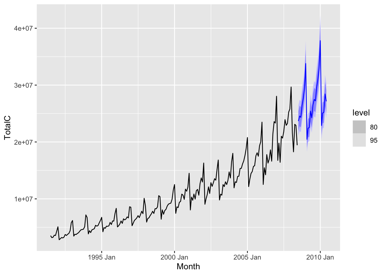

Figure 7.8: Forecasting sales numbers for antidiabetic drugs in Australia using a log transform and a decomposition method.

Prediction intervals usually grow wider as the forecast horizon increases. This is to be expected—the future becomes more uncertain the more distant it is.

7.9.3 Should we trust prediction intervals?

One should be very cautious about taking at face value any prediction interval obtained this way, however, since they express only the uncertainty we have assuming that the model is correct. They thus do not account for the sampling uncertainty in the model parameters as well as the possibility that the model is misspecified, i.e. that it is a poor approximation of the real world mechanism for generating the time series. The latter occurs fairly often, especially for time series for complicated processes such as global temperature, or where feedback and unpredictable human intervention is present.

How to quantify these other sources of uncertainty is an active research area (Yu and Kumbier (2020)). In the meantime, it is better to view prediction intervals heuristically as as lower bounds for how uncertain we are about future values of the time series.

7.9.4 Prediction intervals from bootstrapping

Not all forecasting methods make use of statistical models. When these are absent, we need another method to produce prediction intervals. Enter the bootstrap, which is a general purpose method in statistics for uncertainty quantification. While the boostrap is better known for work with i.i.d. data, it can be adapted to the time series setting too. We will discuss this more in a future chapter and for now refer the interested reader to Chapter 5.5 of Hyndman and Athanasopoulos (2018).

7.10 Evaluating forecast accuracy

Forecasts are only useful if they are reasonably accurate. Accuracy can be formalized via the error between the forecast and the true value of the time series for a future time point, i.e. \[ \hat e_{n+h|n} = x_{n+h} - \hat x_{n+h|n} \] for \(h=1,2,\ldots\).

In order to know how much to trust a given forecast model or how to compare it with other models, we would like to know how to evaluate its accuracy. However, because the future is unknown, we cannot do this directly. We have to somehow estimate it from historical data. This turns out to be much more of a challenge with time series data as opposed to in supervised learning. To explain why, as well as how to overcome these challenges, we take a detour to talk about supervised learning.

7.10.1 LOOCV in supervised learning

In supervised learning, one evaluates model accuracy via sample splitting, either via a single split of the dataset into training and test sets, or via cross-validation. For convenience, let us focus on leave-one-out cross validation (LOOCV). Let us also denote the dataset via \[ \data := \lbrace (x_1,y_1), (x_2,y_2),\ldots (x_n, y_n)\rbrace. \]

Step 1: Train a model \(\hat f_{-i}\) on all except the \(i\)-th data point \((x_i,y_i)\).

Step 2: Evaluate the error \(\hat e_i = \hat f_{-i}(x_i) - y_i\).

Step 3: For \(i=1,2,\ldots,n\), average the squared errors to get \[ \widehat{\text{Err}}_{\text{LOOCV}} = \frac{1}{n}\sum_{i=1}^n \hat e_i^2 \tag{7.3}\]

It is widely accepted that Equation 7.3 is a good approximation of the true out of sample error \[ \mathbb{E}_{x,y}\lbrace (\hat f(x) - y)^2 \rbrace. \] Here, \(\hat f\) is the model trained on thh entire dataset, while the expectation is over a new example \((x,y)\) drawn from the distribution. This approximation relies on several assumptions, the most important of which is that \[ \E_{x_i,y_i}\lbrace (\hat f_{-i}(x_i) - y_i)^2\rbrace \approx \E_{x,y}\lbrace(\hat f_{-i}(x) - y)^2\rbrace \] or, in other words, that the squared error on a held-out example has a similar expectation as that on a new example.

For time series data \(x_1,x_2,\ldots,x_n\), this is not true. The task of predicting a missing past entry \(x_i\) is very different from predicting a future one \(x_{n+h}\). Mathematically, we say that the variables \(x_1,x_2,\ldots,x_n,x_{n+h}\) are not exchangeable. For the same reason, random splits are not appropriate for evaluating the accuracy of forecasting models. We have to use deterministic data splits instead.

7.10.2 Train-test split for time series

The simplest method for splitting time series data is to do a single chronological split, i.e. we select \(x_1,x_2,\ldots,x_m\) to be the training set, and set \(x_{m+1},x_{m+2},\ldots,x_n\) to be the test set. Let us illustrate this process using the antidiabetic drug sales time series data. We first create a training set comprising the first 80% time points.

diabetes_train <- diabetes |> 
    slice_head(n = round(nrow(diabetes) * 0.8))

Here, we used the function slice_head(), but there are several other functions that can be used to filter for subsets of the time points, such as filter(), filter_index(), or variants of slice().

Next, we need to pick an error metric to evaluate the forecast errors. The two most common metrics in regression are mean squared error (MSE) and mean absolute error (MAE), which are defined for time series forecasts as follows: \[ \text{MSE} = \frac{1}{n-m}\sum_{t=m+1}^n \hat e_{t|m}^2, \] \[ \text{MAE} = \frac{1}{n-m}\sum_{t=m+1}^n \left|\hat e_{t|m}\right|. \] We also sometimes take the square root of MSE to get root mean squared error (RMSE).

On the other hand, both MSE and MAE depend on the units of the original time series. We cannot tell based on the raw value of MSE or MAE whether the forecast model is accurate unless we also knew the values taken by the original time series. To overcome this problem, a common strategy is to rescale the errors by a data-dependent quantity. In this way, MSE can be rescaled to obtain the \(R^2\) statistic, which compares the accuracy of the fitted model with that of a constant model. Hyndman and Athanasopoulos (2018) recommends using what they call scaled errors. These compare the model’s errors on the test set with those of the naive method on the training set. More precisely, we define the mean squared scaled error and the mean absolute scaled error as follows: \[ \text{MSSE} = \frac{\text{MSE}}{\frac{1}{m-1}\sum_{t=2}^m (x_{t}-x_{t-1})^2}, \] \[ \text{MASE} = \frac{\text{MAE}}{\frac{1}{m-1}\sum_{t=2}^m \left| x_{t}-x_{t-1}\right|}. \]

Let us now compare the accuracy of all the methods we have seen so far for forecasting antidiabetic drug sales.

diabetes_fit <- diabetes_train |>
    model(
        Mean = MEAN(TotalC),
        Naive = NAIVE(TotalC),
        SeasonalNaive = SNAIVE(TotalC),
        LinearTrend = TSLM(TotalC ~ trend()),
        StlModel = decomposition_model(
            STL(log(TotalC)),
            TSLM(season_adjust ~ trend()))
    )

diabetes_fc <- diabetes_fit |> 
    forecast(h = 41)

diabetes_fc |> autoplot(diabetes, level = NULL)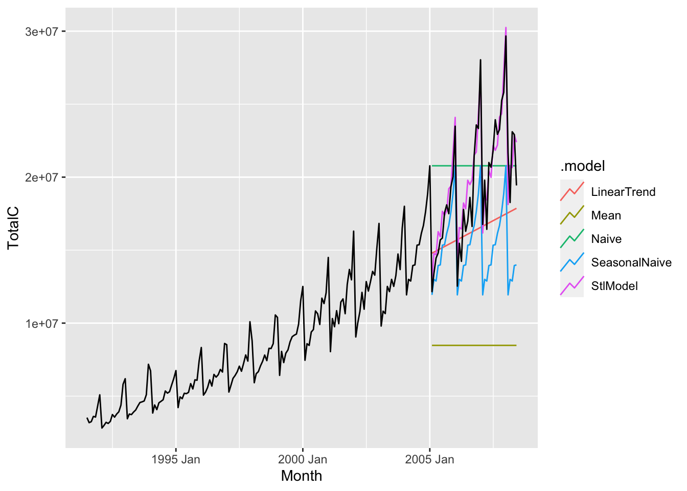

Figure 7.9: Forecasting sales numbers for antidiabetic drugs in Australia using various methods.

From the figure, it seems that the decomposition method is the most accurate. We can verify this by applying the accuracy() function to the fable diabetes_fc.

diabetes_fc |>
    accuracy(diabetes) |>
    select(.model, RMSSE, MASE, RMSE, MAE) |>
    arrange(MASE)

# A tibble: 5 × 5
  .model        RMSSE  MASE      RMSE       MAE
  <chr>         <dbl> <dbl>     <dbl>     <dbl>
1 StlModel       1.32  1.29  1562197.  1267703.
2 Naive          3.67  3.71  4322508.  3645427.
3 LinearTrend    4.06  3.76  4789798.  3687677.
4 SeasonalNaive  4.40  4.34  5186466.  4256436.
5 Mean           9.99 11.2  11783794. 11035335.

The MASE and RMSSE values verify our conclusion that the decomposition method gives the most accurate forecasts.

7.10.3 Time series cross-validation

We have already argued that the task of predicting a missing past entry \(x_i\) of a time series is different from predicting a future one \(x_{n+h}\). Similarly, predicting future values at different time horizons can be different tasks: A forecaster that excels at forecasting demand for durian tomorrow may not be good at predicting demand a month in the future. Mathematically, \(\hat e_{n+h|n}\) and \(\hat e_{n+h'|n}\) may and often do have different distributions for \(h \neq h'\).

We are often in forecasting a specific time horizon so that we can make decisions appropriately. For instance, a supermarket chain would probably be most interested in forecasting the demand for durian a week into the future so that they could manage their inventory today. On the other hand, performing a single train-test split aggregates the error \(\hat e_{m+h|m}\) over all time horizons in the test set, and hence may not directly measure the accuracy for the specific forecasting task at hand.

To resolve this, one may perform time series cross-validation, also known as “evaluation on a rolling forecasting origin”. As in cross-validation for supervised learning, we use multiple splits to create multiple pairs of training and test sets. Unlike in supervised learning, however, the training sets are not random, nor are they even of the same size. Instead, they are overlapping, each comprising all time series values before a certain time point. This is best illustrated by the following diagram, taken from Hyndman and Athanasopoulos (2018).

Figure 7.10: Time series cross-validation for 4-step-ahead forecasts

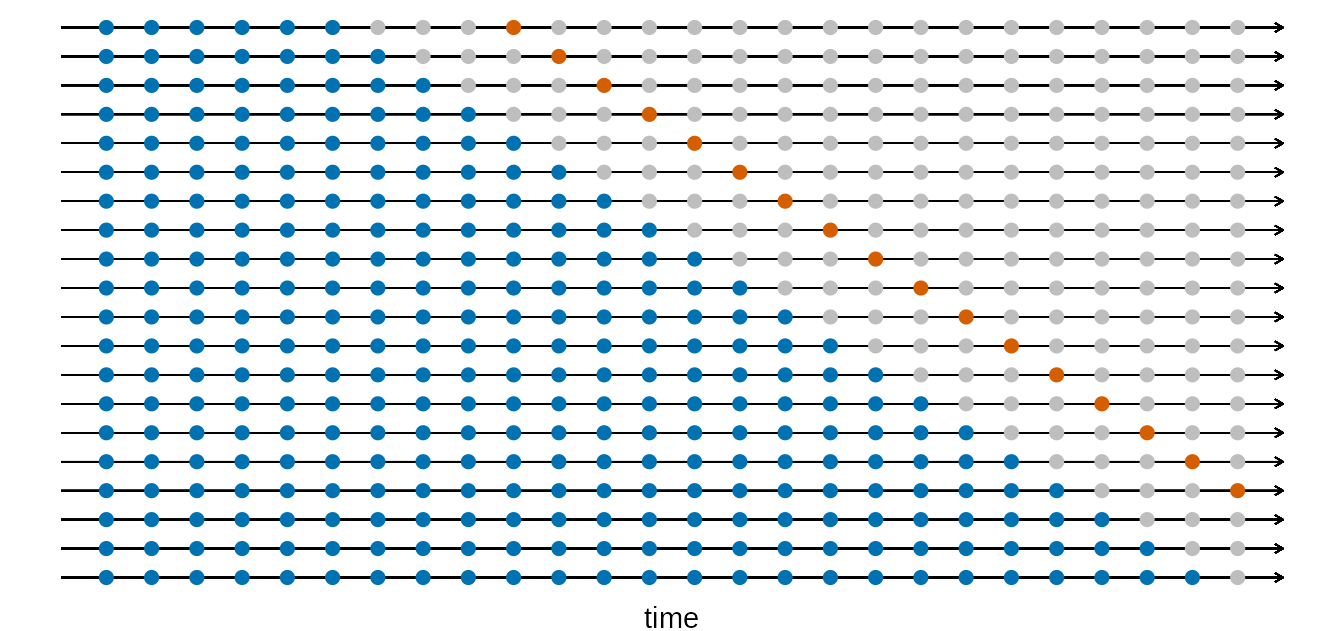
Here, each row corresponds to a training set, test set pair, with the former colored in blue, while the latter is colored in red. Time belonging to neither train nor test sets are grayed out. Note that in this example, we assume that we are interested in evaluating the accuracy of 4-step ahead forecasts, which is why each test set comprises a single time point 4 units after the last measurement in the training set.

We now describe how to implement time series cross-validation using tsibble, again using the antidiabetic drug sales data as a working example. Suppose we are interested in 6 month ahead forecasts. First, we use stretch_tsibble() to create a tsibble containing all of the training sets. Here, .init indicates the minimum size of a training set, and .step refers to the difference in size of consecutive training sets. In particular, .init = 120, .step = 1 implies that we will have training sets of size \(120, 121, 122, \ldots\).⁴

diabetes_cv <- diabetes |> stretch_tsibble(.init = 120, .step = 1)
diabetes_cv

# A tsibble: 13,770 x 4 [1M]
# Key:       .id [85]
      Month  TotalC  Cost   .id
      <mth>   <dbl> <dbl> <int>
 1 1991 Jul 3526591  3.53     1
 2 1991 Aug 3180891  3.18     1
 3 1991 Sep 3252221  3.25     1
 4 1991 Oct 3611003  3.61     1
 5 1991 Nov 3565869  3.57     1
 6 1991 Dec 4306371  4.31     1
 7 1992 Jan 5088335  5.09     1
 8 1992 Feb 2814520  2.81     1
 9 1992 Mar 2985811  2.99     1
10 1992 Apr 3204780  3.20     1
# ℹ 13,760 more rows

Note that diabetes_cv has a new key column called .id. This indicates which training set the measurement belongs to. Since there are 85 values of .id, this means that there are 85 training sets.

Next, we fit the same suite of models to this data, use these models to forecast 6 steps ahead, and then evaluate the accuracy.

diabetes_fit <- diabetes_cv |>
    model(
        Mean = MEAN(TotalC),
        Naive = NAIVE(TotalC),
        SeasonalNaive = SNAIVE(TotalC),
        LinearTrend = TSLM(TotalC ~ trend()),
        StlModel = decomposition_model(
            STL(log(TotalC)),
            TSLM(season_adjust ~ trend()))
    )

diabetes_fc <- diabetes_fit |>
    forecast(h = 6)

As before, forecast(h = 6) produces forecasts for each model for the next 6 time steps. Since we only want to evaluate the accuracy of the forecast at horizon \(h = 6\), we need to perform some additional steps.

diabetes_fc |>
1    group_by(.id) |>
    mutate(h = ((row_number() - 1) %% 6) + 1) |>
    ungroup() |>
2    filter(h == 6) |>
3    as_fable(response = "TotalC", distribution = TotalC) |>
    accuracy(diabetes) |>
    select(.model, RMSSE, MASE, RMSE, MAE) |>
    arrange(MASE)

1

These three lines add an addition column to the fable, denoting the horizon of the forecast corresponding to that row.

2

We filter for only the forecasts that are at horizon \(h = 6\).

3

The operations on the previous lines have produced a table that is no longer of the fable class. We hence have to convert it back to a fable again.

# A tibble: 5 × 5
  .model        RMSSE  MASE     RMSE      MAE
  <chr>         <dbl> <dbl>    <dbl>    <dbl>
1 StlModel      0.769 0.816 1329482. 1057465.
2 SeasonalNaive 1.41  1.50  2435712. 1937908.
3 LinearTrend   2.04  1.98  3521441. 2561206.
4 Naive         2.40  2.80  4146710. 3629952.
5 Mean          5.33  6.50  9212715. 8424294.

Again, we see that the decomposition forecasting method has the best performance. Notice also that all methods have better RMSSE compared to the single train-test split. This is unsurprising as the test error for the single split involved evaluting forecasts up to 41 steps ahead, as opposed to just 6 steps ahead for time series cross-validation.

7.10.4 Evaluating distributional forecasts

So far, we have discussed how to evaluate the accuracy of point forecasts. There are also methods for evaluating the accuracy of distributional forecasts, but these are beyond the scope of this course. We refer the interested reader to Chapter 5.9 of Hyndman and Athanasopoulos (2018).

Altieri, Nick, Rebecca L Barter, James Duncan, Raaz Dwivedi, Karl Kumbier, Xiao Li, Robert Netzorg, et al. 2020. “Curating a COVID-19 Data Repository and Forecasting County-Level Death Counts in the United States.” arXiv Preprint arXiv:2005.07882.

Hyndman, Rob J, and George Athanasopoulos. 2018. Forecasting: Principles and Practice. OTexts.

Ke, Guolin, Qi Meng, Thomas Finley, Taifeng Wang, Wei Chen, Weidong Ma, Qiwei Ye, and Tie-Yan Liu. 2017. “LightGBM: A Highly Efficient Gradient Boosting Decision Tree.” In Advances in Neural Information Processing Systems. Vol. 30. Curran Associates, Inc. https://proceedings.neurips.cc/paper/2017/hash/6449f44a102fde848669bdd9eb6b76fa-Abstract.html.

Makridakis, Spyros, Evangelos Spiliotis, and Vassilios Assimakopoulos. 2022. “M5 Accuracy Competition: Results, Findings, and Conclusions.” International Journal of Forecasting 38 (4): 1346–64.

Yu, Bin, and Karl Kumbier. 2020. “Veridical Data Science.” Proceedings of the National Academy of Sciences 117 (8): 3920–29. https://doi.org/10.1073/pnas.1901326117.

---

1. seasonal_adjust and season_year are the names of columns in the tsibble returned by applying the function components() to a time series decomposition model. Depending on the type of seasonality, the seasonal component returned by STL may have a different name, and there may even be multiple seasonal components.

2. See for instance Altieri et al. (2020).

3. A good resource is the website Papers with Code, which shows several benchmark datasets as well as the performance of different forecasting methods on these datasets. Do note, however, that this is an incomplete list.

4. For statistical purposes, it is always better to calculate the error over more training sets. However, this can be very computationally expensive to run. If your computer takes a long time to execute time series cross-validation, try increasing .step to a larger value.