cowtemp <- fma::cowtemp |>
    as_tsibble() |>
    rename(Day = index,
              Temp = value)
cowtemp |> autoplot(Temp)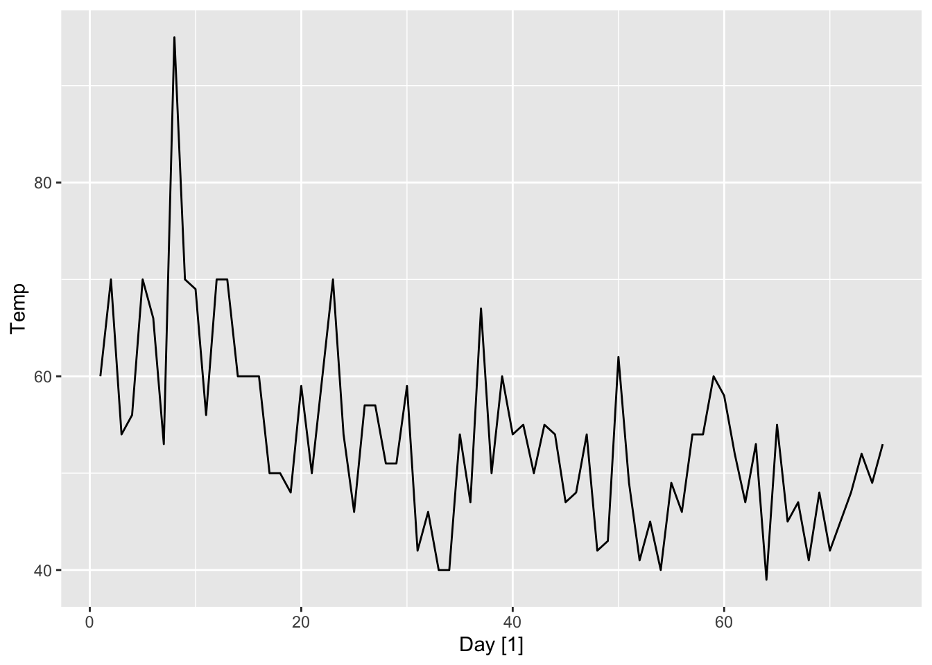
Exponential smoothing is a family of forecasting methods that make use of (exponentially) weighted averages of past observations in their forecast equations. These are easy to fit and yet often very powerful, and are therefore used extensively in many applications.
Recall the forecast formulas for the mean method and the naive method. The former uses the mean of all the observed values, while the latter uses only the most recent observation. The former has low variance but potentially high bias, whereas the latter has high variance but potentially low bias. It is useful to have a method that is intermediate between these two extremes. More precisely, we would like to use multiple previous observations, but at the same time, prioritize those that are more recent. An elegant solution is provided by simple exponential smoothing (SES), which uses exponentially weighted averages, i.e. \[ \hat{x}_{n+h|n} = \alpha \sum_{j=0}^{n-1}(1-\alpha)^j x_{n-j} + (1-\alpha)^n l_0. \tag{8.1}\]
Note that the weights indeed sum to one: \[ \alpha \sum_{j=0}^{n=1} (1-\alpha)^j + (1-\alpha)^n = \frac{\alpha(1 - (1-\alpha)^n)}{1 - (1-\alpha)} + (1-\alpha)^n = 1. \]
\(\alpha \in [0,1]\) and \(l_0 \in \mathbb{R}\) are the parameters of the method, and are fitted by minimizing the sum of squared errors:
\[ \text{SSE}(\alpha,l_0) = \sum_{t=1}^n (x_t - \hat x_{t|t-1})^2. \tag{8.2}\]
Note that when \(\alpha = 1\), SES is equivalent to the naive method, while when \(\alpha = 0\), it is equivalent to the mean method. More generally, the smaller the value of \(\alpha\), the slower the rate of decay of the weights.
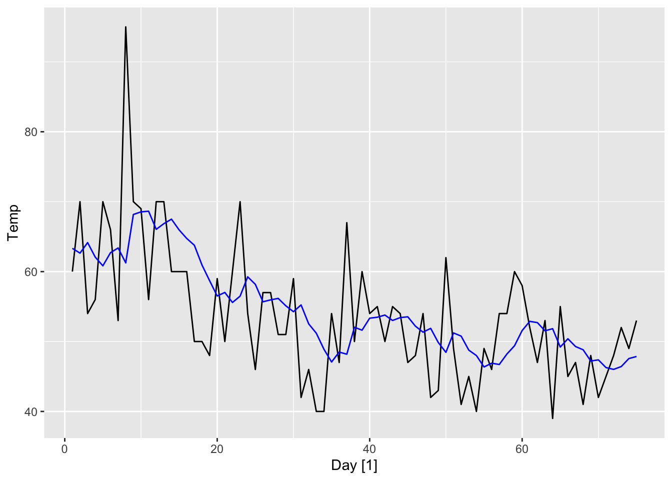
Let us now apply this method to a data example and compare its performance to that of the simple forecasting methods we have learnt so far. To this end, consider the time series cowtemp measuring the daily morning temperature of a cow. This dataset is found in the fma package and its time and ACF plots are shown below.
cowtemp <- fma::cowtemp |>
as_tsibble() |>
rename(Day = index,
Temp = value)
cowtemp |> autoplot(Temp)
cowtemp |>
    ACF(Temp) |>
    autoplot()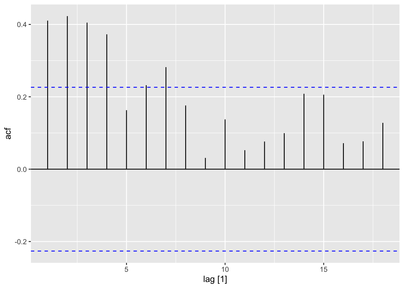
We now fit SES and inspect the model parameters.
cow_fit <- cowtemp |>
    model(SES = ETS(Temp ~ error("A") + trend("N") + season("N")))

cow_fit |> tidy()
# A tibble: 2 × 3
.model term estimate
<chr> <chr> <dbl>
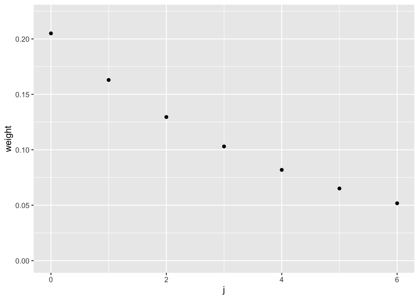
1 SES alpha 0.205
2 SES l[0] 63.3 The syntax for fitting SES may seem somewhat confusing at the moment. We will explain it more later in the chapter. For now, we note that the fitted value for \(\alpha\) is \(0.205\), which gives a fairly slow rate of decay. The resulting weights are plotted below in Figure 8.3.
To make sense of this, we return to the time and ACF plots of cowtemp. The ACF plot shows decaying autocorrelation behavior, meaning that past observations lose relevancy the older they are. On the other hand, the time plot shows that the time series is not a random walk—it seems to comprise fluctuations of constant variance around a slightly decreasing trend. As such, it is better to forecast with a window of past observations to average out some of the irrelvant noise.
We now compare the cross-validation accuracy of SES against that of the mean, naive, drift, and linear trend methods. We see that SES indeed has the smallest RMSSE and MASE.
cow_cv <- cowtemp |>
    stretch_tsibble(.init = 10, .step = 1) |>
    model(Naive = NAIVE(Temp),
          Mean = MEAN(Temp),
          Drift = NAIVE(Temp ~ drift()),
          LinearTrend = TSLM(Temp ~ trend()),
          SES = ETS(Temp ~ error("A") + trend("N") + season("N")))

cow_fc <- cow_cv |> forecast(h = 1)

cow_fc |>
    accuracy(cowtemp) |>
    select(.model, RMSSE, MASE) |>
    arrange(RMSSE)
# A tibble: 5 × 3
.model RMSSE MASE
<chr> <dbl> <dbl>
1 SES 0.725 0.789
2 LinearTrend 0.771 0.826
3 Naive 0.832 0.888
4 Drift 0.848 0.909
5 Mean 0.897 1.01 Finally, we show the difference in forecasts for the mean, naive, and SES methods when fitted to only the first 64 days:
cowtemp |>
    slice_head(n = 64) |>
    model(Mean = MEAN(Temp),
          Naive = NAIVE(Temp),
          SES = ETS(Temp ~ error("A") + trend("N") + season("N"))) |>
    forecast(h = 11) |>
    autoplot(cowtemp, level = NULL)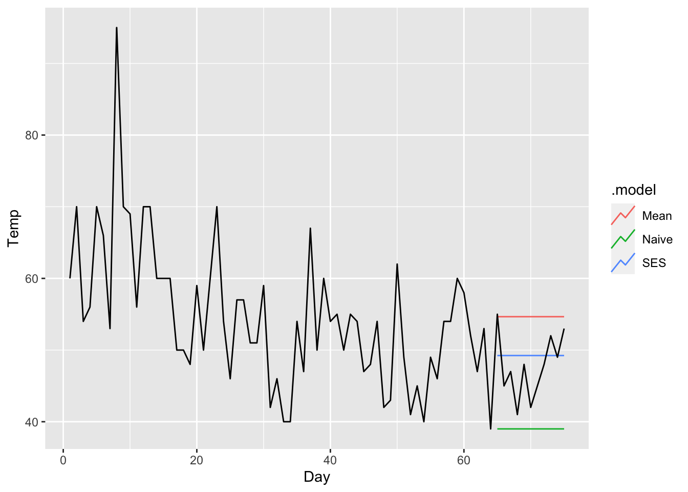
There is another way to view SES, which is more amenable to generalization. That is, we break down Equation 8.1 into two steps, with the first step comprising a transformation into a new time series \((l_t)\), defined recursively via a smoothing equation: \[ \begin{split} l_t & = \alpha x_t + (1-\alpha)l_{t-1} \\ & = l_{t-1} + \alpha(x_t - l_{t-1}). \end{split} \tag{8.3}\] \(l_t\) is called the level (or the smoothed value) of \((x_t)\) at time \(t\) and is obtained from the previous level by adding an \(\alpha\)-fraction of the difference between the new observation \(x_t\) and the previous level \(l_{t-1}\). Again, the smaller \(\alpha\) is, the smaller the influence of each new observation on the level, or in other words, the more the fluctuations of \((x_t)\) are smoothed out. Naturally \(\alpha\) is called the smoothing parameter.
In the second step, we make use of the level to make a forecast: \[ \hat x_{n+h|n} = l_n. \tag{8.4}\] Using induction, one may easily check that Equation 8.3 and Equation 8.4 are equivalent to Equation 8.1.
The following plot shows the difference between the original time series \((x_t)\) for our example and its level \((l_t)\).
Inspecting Equation 8.4, we see that SES produces a constant forecast (i.e. it predicts the same value \(l_n\) for any forecast horizon \(h\)). When the time series has a clear trend, however, we would like to be able to extrapolate it.
We have seen that the linear trend or the drift method are able to extrapolate trends. On the other hand, both these methods assume that the trend is linear, which is a strong assumption not satisfied by most real world time series. While it is possible to assume a naive trend method that makes use of only the two most recent values, we would again like to achieve a happy medium between the two extremes by using some form of exponential smoothing.
Holt’s linear trend method does exactly that. It generalizes on Equation 8.3 to get two new time series \((l_t)\) and \((b_t)\), where \(l_t\) is still the level of the time series at time \(t\), while \(b_t\) is the current best estimate for the trend at time \(t\). These are defined by the smoothing equations: \[ l_t = \alpha x_t + (1-\alpha)(l_{t-1} + b_{t-1}), \tag{8.5}\] \[ b_t = \beta^*(l_t - l_{t-1}) + (1-\beta^*)b_{t-1}. \tag{8.6}\] To update the level, we first extrapolate the previous value \(l_{t-1}\) using the previous trend estimate \(b_{t-1}\) and then form a weighted average between this value and that of the new observation \(x_t\).1 The trend estimate is then updated by taking a weighted average between the previous estimate \(b_{t-1}\) and the change in level \(l_t - l_{t-1}\). Here, \(\alpha, \beta^* \in [0, 1]\) are the smoothing parameters for the level and trend respectively.2 As with SES, they are both estimated, together with \(l_0\) and \(b_0\), by minimizing the sum of squared errors Equation 8.2. Finally, the forecast is given by linear extrapolation using the last calculated value for the trend: \[ \hat x_{n+h|n} = l_n + h b_n. \tag{8.7}\]
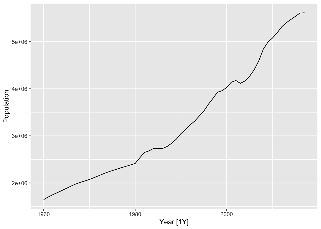
We now compare the accuracy of Holt’s linear trend method with that of SES, as well as the drift and linear trend methods, when used to forecast for the Singapore population time series. The time plot and the CV accuracy is shown below. As expected, Holt’s linear trend method has the best accuracy.
sg_cv <- sg_pop |>
    stretch_tsibble(.init = 10, .step = 1) |>
    model(Drift = NAIVE(Population ~ drift()),
          LinearTrend = TSLM(Population ~ trend()),
          Holt = ETS(Population ~ error("A") + trend("A") + season("N")),
          SES = ETS(Population ~ error("A") + trend("N") + season("N")))

sg_fc <- sg_cv |> forecast(h = 1)

sg_fc |>
    accuracy(sg_pop) |>
    select(.model, RMSSE, MASE) |>
    arrange(RMSSE)
# A tibble: 4 × 3
.model RMSSE MASE
<chr> <dbl> <dbl>
1 Holt 0.581 0.512
2 Drift 0.647 0.555
3 SES 1.07 1.07
4 LinearTrend 3.35 3.05 While Holt’s linear trend method forecasts by linearly extrapolating the trend (Equation 8.7), linear trends rarely persist indefinitely. As such, Holt’s method can lead to large errors when forecasting over long time horizons. One idea to overcome this is to modify the method using a damping parameter \(\phi \in (0,1)\). Thew new smoothing and forecast equations are:
\[ l_t = \alpha x_t + (1-\alpha)(l_{t-1} + \phi b_{t-1}), \tag{8.8}\] \[ b_t = \beta^*(l_t - l_{t-1}) + (1-\beta^*) \phi b_{t-1}. \tag{8.9}\]
\[ \hat x_{n+h|n} = l_n + (\phi + \phi^2 + \cdots + \phi^h)b_n. \tag{8.10}\]
Here, we see that we have used \(\phi\) in both the smoothing equations to dampen the influence of the previous trend estimate \(b_{t-1}\). In the forecast equation, while the trend is still extrapolated, its slope is attenuated by a factor of \(\phi\) as the forecast horizon increases. Indeed, one may show that the forecasts asymptote to a constant value: \[ \lim_{h \to \infty} \hat x_{n+h|n} = l_n + \frac{\phi}{1 - \phi} b_n. \] One can check that when \(\phi = 1\), this method is the same as Holt’s linear trend method, while when \(\phi = 0\), this is equivalent to SES. Note that \(\phi\) is usually estimated from the data together with the other parameters, but can also be set manually.
We now apply the damped trend method, with several choices of \(\phi\), to the Singapore population time series. We fit the models on the observations up to 2007, and forecast for the next 20 years.
sg_pop |>
    slice_head(n = 48) |>
    model(Holt = ETS(Population ~ error("A") + trend("A") + season("N")),
          Damped95 = ETS(Population ~ error("A") + trend("Ad", phi = 0.95) + season("N")),
          Damped90 = ETS(Population ~ error("A") + trend("Ad", phi = 0.9) + season("N")),
          Damped80 = ETS(Population ~ error("A") + trend("Ad", phi = 0.8) + season("N"))
    ) |>
    forecast(h = 20) |>
    autoplot(sg_pop, level = NULL)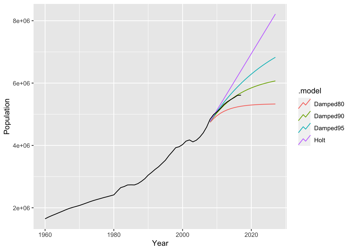
From Figure 8.7, we see that the undamped Holt linear trend method is overly optimistic. It projects a population of greater than 8 million by 2024, which is clearly unrealistic. As \(\phi\) becomes smaller, the forecasts asymptote more and more quickly to a flat line, with the choice \(\phi = 0.9\) seemingly the best in this scenario
We now compare the cross-validation performance of these methods, together with SES, using two different forecasting horizons.
sg_cv <- sg_pop |>
    stretch_tsibble(.init = 10, .step = 1) |>
    model(Holt = ETS(Population ~ error("A") + trend("A") + season("N")),
          Damped95 = ETS(Population ~ error("A") + trend("Ad", phi = 0.95) + season("N")),
          Damped90 = ETS(Population ~ error("A") + trend("Ad", phi = 0.9) + season("N")),
          Damped80 = ETS(Population ~ error("A") + trend("Ad", phi = 0.8) + season("N")),
          SES = ETS(Population ~ error("A") + trend("Ad") + season("N")))

sg_fc1 <- sg_cv |> forecast(h = 1)

sg_fc1 |>
    accuracy(sg_pop) |>
    select(.model, RMSSE, MASE) |>
    arrange(RMSSE)
# A tibble: 5 × 3
.model RMSSE MASE
<chr> <dbl> <dbl>
1 Damped80 0.523 0.487
2 Damped90 0.529 0.466
3 Damped95 0.548 0.486
4 Holt 0.581 0.512
5 SES 0.625 0.539sg_fc5 <- sg_cv |> forecast(h = 5)
sg_fc5 |>
accuracy(sg_pop) |>
select(.model, RMSSE, MASE) |>
arrange(RMSSE)# A tibble: 5 × 3
.model RMSSE MASE
<chr> <dbl> <dbl>
1 Damped90 1.98 1.53
2 Damped95 2.03 1.57
3 Damped80 2.04 1.63
4 SES 2.09 1.61
5 Holt 2.11 1.59In both cases, damping seems to improve over both SES and Holt’s linear trend method, although the optimal level of damping varies. This also shows that damping can also help with short-term forecasts.
As we have seen, many real world datasets contain seasonality. While the methods introduced in the previous sections do not account for seasonality, it is relatively straightforward to extend them to do so using ideas from time series decomposition. Just as there are additive and multiplicative decompositions, there are additive and multiplicative approaches to incoporating seasonality into exponential smoothing. Both are known as versions of Holt-Winters’ method.
Given a period \(p\) for the seasonality, the smoothing equations for the additive method are shown below:
\[ l_t = \alpha (x_t - s_{t-p}) + (1-\alpha)(l_{t-1} + b_{t-1}), \tag{8.11}\] \[ b_t = \beta^*(l_t - l_{t-1}) + (1-\beta^*) b_{t-1}, \tag{8.12}\]
\[ s_t = \gamma(x_t - l_{t-1} - b_{t-1}) + (1-\gamma) s_{t-p}. \tag{8.13}\] Here, we keep track of three components of \((x_t)\): The level \((l_t)\), the trend \((b_t)\), and the seasonal component \((s_t)\). To update the level, we first extrapolate the level \(l_{t-1}\) using the previous trend estimate \(b_{t-1}\) and then form a weighted average between this value and that of the seasonally adjusted new observation \(x_t - s_{t-p}\). The trend estimate is then updated in the same way as in Holt’s linear trend method (Equation 8.6). Finally, we update the seasonal component by using a weighted average of the seasonal component one period ago and the detrended new observation \(x_t - l_{t-1} - b_{t-1}\). Note that we now have \(5 + p\) parameters to estimate: \(\alpha, \beta^*, \gamma, l_0, b_0\), and \(s_0,s_{-1},\ldots,s_{p-1}\). Finally, the forecast equation is: \[ \hat x_{n+h|n} = l_n + h b_n + s_{n - p + (h ~\text{mod}~p)}. \tag{8.14}\]
The multiplicative method is similar to the additive method, except we view the seasonal component as adjusting the the non-seasonal components multiplicatively. This is useful when the seasonal fluctuations are roughly proportional to the level of the time series. The smoothing and forecast equations are as follows:
\[ l_t = \alpha \frac{x_t}{s_{t-p}} + (1-\alpha)(l_{t-1} + b_{t-1}), \] \[ b_t = \beta^*(l_t - l_{t-1}) + (1-\beta^*) b_{t-1}, \]
\[ s_t = \gamma \frac{x_t}{l_{t-1} + b_{t-1}} + (1-\gamma) s_{t-p}. \]
\[ \hat x_{n+h|n} = (l_n + h b_n)s_{n - p + (h ~\text{mod}~p)}. \]
Note that this is not equivalent to applying a log transform on \(x_t\) followed by the additive method. In particular, each state is updated additively instead of multiplicatively.
Just as with Holt’s linear trend method, it is often useful to damp the influence of the trend. One may do this with both the additive and multiplicative forms of Holt-Winters, with the equations for the multiplicative form shown below:
\[ l_t = \alpha \frac{x_t}{s_{t-p}} + (1-\alpha)(l_{t-1} + \phi b_{t-1}), \] \[ b_t = \beta^*(l_t - l_{t-1}) + (1-\beta^*) \phi b_{t-1}, \]
\[ s_t = \gamma \frac{x_t}{l_{t-1} + \phi b_{t-1}} + (1-\gamma) s_{t-p}. \]
\[ \hat x_{n+h|n} = (l_n + (\phi + \phi^2 + \cdots + \phi^h) b_n)s_{n - p + (h ~\text{mod}~p)}. \]
Note that only the trend component is damped, while the seasonal component remains undamped. As such, the forecasts do not asymptote to a constant forecast, but instead have persistent seasonality.
We now apply both the additive and multiplicative forms of Holt-Winters to the time series of tourist arrivals to Australia from Japan from the aus_arrivals dataset. We show a time plot of the forecasts fitted with the last 5 years of the time series omitted.
aus_arrivals |>
    filter(Origin == "Japan") |>
    slice_head(n = 107) |>
    model(SNaive = SNAIVE(Arrivals ~ drift()),
          Additive = ETS(Arrivals ~ error("A") + trend("A") + season("A")),
          Multiplicative = ETS(Arrivals ~ error("M") + trend("A") + season("M"))
    ) |>
    forecast(h = 20) |>
    autoplot(aus_arrivals, level = NULL)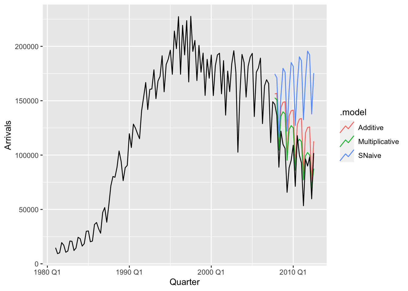
We see that the seasonal naive method with drift completely misses the fact that the trend has changed after 1995. Both the additive and multiplicative Holt-Winters methods are able to pick up on this. On the other hand, the seasonality seems to be accounted for more accurately via the multiplicative method, while it is overestimated using the additive method as the number of tourists decreases.
Finally, we compare the performance of these methods, together with the damped versions of Holt-Winters methods, using cross-validation using two different forecasting horizons. In this case, it seems that the damped additive method has the best performance.
aus_cv <- aus_arrivals |>
    filter(Origin == "Japan") |>
    stretch_tsibble(.init = 10, .step = 1) |>
    model(SNaive = SNAIVE(Arrivals ~ drift()),
          Additive = ETS(Arrivals ~ error("A") + trend("A") + season("A")),
          Multiplicative = ETS(Arrivals ~ error("M") + trend("A") + season("M")),
          AdditiveDamped = ETS(Arrivals ~ error("A") + trend("Ad") + season("A")),
          MultiplicativeDamped = ETS(Arrivals ~ error("M") + trend("Ad") + season("M"))
    )

aus_fc1 <- aus_cv |>
    forecast(h = 5)

aus_fc1 |>
    accuracy(aus_arrivals) |>
    select(.model, RMSSE, MASE) |>
    arrange(RMSSE)
# A tibble: 5 × 3
.model RMSSE MASE
<chr> <dbl> <dbl>
1 AdditiveDamped 0.973 0.995
2 Additive 1.02 1.03
3 Multiplicative 1.07 1.04
4 MultiplicativeDamped 1.13 1.07
5 SNaive 1.16 1.19 aus_fc5 <- aus_cv |>
forecast(h = 5)
aus_fc5 |>
accuracy(aus_arrivals) |>
select(.model, RMSSE, MASE) |>
arrange(RMSSE)# A tibble: 5 × 3
.model RMSSE MASE
<chr> <dbl> <dbl>
1 AdditiveDamped 0.973 0.995
2 Additive 1.02 1.03
3 Multiplicative 1.07 1.04
4 MultiplicativeDamped 1.13 1.07
5 SNaive 1.16 1.19 fableWe now explain the code syntax used for specifying exponential smoothing methods in fable, while at the same time providing a taxonomy of these methods. The general recipe is to write
ETS(X ~ error(O1) + trend(O2) + season(O3))Here, X is the column name of the time series being modeled O2 is set to be one of "A", "Ad", or "N", depending on whether a linear trend, a damped linear trend, or no trend component is to be included in the model. O3 is set to be one of "A", "M", or "N", depending on whether additive, multiplicative, or no seasonal component is to be included. Finally, O1 is set to be either "A" or "M" depending on whether the “noise” is to be additive or multiplicative. This also explains the term ETS, which stands for Error, Trend, Seasonal.
To understand the choices for O1 further, recall that in Section 7.6, we saw that the simple forecasting methods we have learnt are associated with statistical models. The exponential smoothing methods are no different. Indeed, each of them arises from a state space model, which are models that include latent variables which evolve over time. The components \((l_t)\), \((b_t)\), and \((s_t)\) are precisely our best estimates of these latent variables.
We will discuss the evolution equations for these models, as well as state space models more generally, in part 2 of the book. For now, note that these models include a noise term for the observations that can be either additive or multiplicative in nature. For the same choice of other parameters values (\(\alpha\), \(\beta^*\), etc.), this choice does not affect the point forecasts. On the other hand, it affects the distributional forecast.3 Furthermore, if multiplicative noise is chosen, the parameters are estimated using an objective function that is different from the sum of squared errors (Equation 8.2), arising from maximum likelihood.
While each term O1, O2, and O3 can be freely set, some combinations can lead to numerical instabilities and should be avoided. These are ETS(A, N, M), ETS(A, A, M), and ETS(A, Ad, M). Lastly, note that when the time series contains zeros or negative values, multiplicative errors are not feasible.
If one of the terms is not specified in the formula, ETS automatically performs model selection to decide on the most appropriate choice for that term. We will discuss model selection in more detail in part 2 of the book.
This can also be seen as adding to the one-step-forecast \(l_{t-1} + b_{t-1}\) an \(\alpha\) fraction of the difference between the value of the new observation \(x_t\) and that of the forecast.↩︎
We follow the convention of Hyndman and Athanasopoulos (2018) in denoting the smooothing parameter of the trend using \(\beta^*\) instead of \(\beta\).↩︎
As before, having a statistical model allows us to produce distributional forecasts and prediction intervals.↩︎