\(\textnormal{ARMA}(p,q)\) models are used to model stationary time series. However, many real-world time series are not stationary. Hence, following the Box-Jenkins approach to time series modeling (see Section 9.7), one first transforms a time series to make it stationary, before modeling the transformed time series using \(\textnormal{ARMA}(p,q)\) models.
There are multiple choices of transformations. The trend and seasonality can be estimated directly and removed from the time series. Another method is to perform differencing.
12.1.1 Types of differencing
Given a time series \((X_t)\), its difference can be written as \[
Y_t = (I-B)X_t.
\] More generally, we can take differences multiple times, and \[
Y_t = (I-B)^d X_t
\] is called the \(d\)-th order difference of the time series.
Finally, instead of taking the difference between consecutive values of the time series, we can take differences of values that are some lag \(m\) apart, i.e. \(Y_t = X_t - X_{t-m}\). This is called the seasonal difference, as it is usually applied to seasonal data, with \(m\) equal to the period of ths seasonality. It can be written in operator form as \[
Y_t = (I - B^m)X_t.
\]
As we will soon see, both differences and seasonal differences can be applied simultaneously to the same time series.
12.1.2 Effects of differencing
Differencing can resolve a few types of non-stationarity. First, if \((X_t)\) is already stationary, then any difference (or seasonal difference) of \((X_t)\) remains stationary (check this). On the other hand, if we have \[
X_t = A_t + Z_t
\tag{12.1}\] for a non-stationary \(A_t\), then differencing can help to get rid of \(A_t\):
Polynomial trend. If \((X_t)\) has a polynomial trend, i.e. \(A_t = f(t)\), where \(f\) is a degree \(d\) polynomial, then \((I-B)^d A_t = \alpha\) for some \(\alpha \in \R\).1
Proof. Prove this by induction, with the base case \(d = 0\) trivial. For any \(d+1\) degree polynomial \(f(t)\), it is easy to see that \(f(t+1) - f(t)\) is of degree at most \(d\), which completes the induction step. \(\Box\)
Constant seasonality. If \((X_t)\) has constant seasonality, i.e. \(A_{t} = A_{t-m}\) for all \(t\), then \[
(I-B^m)A_t = 0.
\]
Any \((X_t)\) that satisfies Equation 12.1 is called trend stationary. We have already learnt other methods for estimating and removing the non-stationary component \((A_t)\). However, as we have seen, there are other types of non-stationarity that are even more intrinsic to \((X_t)\) and which can only be resolved by differencing.
For instance, if \((X_t)\) is a random walk, then \((I-B)X_t = W_t\), which is stationary. More generally, differencing helps to deal with the existence of unit roots, which we will define shortly.
Differencing and ARMA modeling form a coherent mathematical framework because of their common use of the backshift operator. Their combination is known as ARIMA modeling and turns out to also be very useful practically. We now introduce this new class of models.
12.2 Introducing ARIMA models
12.2.1 ARIMA
An autoregressive integrated moving average model of order \(p\), \(d\), and \(q\), abbreviated \(\textnormal{ARIMA}(p,d,q)\), is a stochastic process \((X_t)\) such that \((I-B)^d X_t\) is an \(\textnormal{ARMA}(p,q)\) model. It can be written in operator form as \[
\phi(B)(I-B)^dX_t = \alpha + \theta(B) W_t.
\tag{12.2}\] As with \(\textnormal{ARMA}(p,q)\) models, \(\phi(z)\) and \(\theta(z)\) are called the autoregressive and moving average polynomials of the model resepctively. Furthermore, the mean of \((I-B)^dX_t\) is equal to \(\alpha/(1-\phi_1-\phi_2-\cdots-\phi_p)\).
Similar to \(\textnormal{ARMA}(p,q)\) models, \(\textnormal{ARIMA}(p,d,q)\) can also be interpreted as describing dynamical systems perturbed by noise. The order of differencing, \(d\), reflects the minimum order of the derivative at which any interesting dynamics is happening.
Note that while \(\textnormal{ARIMA}(p,d,q)\) models are well-defined for any choice of \(d\), \(d > 2\) leads to too much instability, and is not implemented in fable.
12.2.2 SARIMA
As hinted at by seasonal differencing, both ARMA and ARIMA models can be extended to account for seasonal relationships. To do so, we simply prioritize lags that are multiples of the seasonal period.
A seasonal autoregressive integrated moving average model of order \(p\), \(d\), \(q\), \(P\), \(D\), and \(Q\), with seasonal period \(m\), abbreviated \(\textnormal{ARIMA}(p,d,q)(P,D,Q)_m\), is a stochastic process \((X_t)\) satisfying \[
\Phi(B^m)\phi(B)(I-B^m)^D(I-B)^dX_t = \alpha + \Theta(B^m)\theta(B) W_t.
\]\(\phi(z)\) and \(\theta(z)\) are called the autoregressive and moving average polynomials of the model resepctively, while \(\Phi(z)\) and \(\Theta(z)\) are called the seasonal autoregressive and seasonal moving average polynomials respectively.
One can check that the mean of \((I-B^m)^D(I-B)^dX_t\) is equal to \[
\frac{\alpha}{(1-\phi_1-\phi_2-\cdots-\phi_p)(1 - \Phi_1 - \Phi_2 - \cdots - \Phi_P)}.
\]
For the rest of this chapter, we will focus on explaining ARIMA models, with the understanding that everything discussed generalizes easily to the SARIMA setting.
12.2.3 Examples
Several of the time series models we have already seen are instances of ARIMA models.
Random walk with drift. Random walk with drift (see Equation 9.2) is equivalent to an \(\textnormal{ARIMA}(0,1,0)\) model with a mean term.
Simple exponential smoothing. Simple exponential smoothing is equivalent to forecasting with an \(\textnormal{ARIMA}(0,1,1)\) model. To see this, we start with the latter and derive the forecasting equation. The \(\textnormal{ARIMA}(0,1,1)\) equation is: \[
X_t = X_{t-1} + W_t + \theta W_{t-1},
\] Write \(Y_t = X_t - X_{t-1}\). Suppose invertibility holds, then by solving Equation 11.3, we have \[
\sum_{j=0}^\infty (-\theta)^j Y_{t-j} = W_t.
\] Substituting \(X_t\) back in and using summation by parts, we get
\[\begin{split}
W_t & = \sum_{j=0}^\infty (-\theta)^j (X_{t-j} - X_{t-j-1}) \nonumber\\
& = \sum_{j=0}^\infty ((-\theta)^{j+1}-(-\theta)^j)X_{t-j-1} + X_t \nonumber\\
& = X_t - (1+\theta)\sum_{j=0}^\infty (-\theta)^j X_{t-j-1}.
\end{split}\]
Rearranging, we get \[
X_t = (1+\theta)\sum_{j=0}^\infty (-\theta)^j X_{t-j-1} + W_t.
\] Assuming we observe \(X_1,\ldots,X_n\) and following the logic of Section 11.4, the truncated forecast is \[
\hat X_{n+1|n} = (1+\theta)\sum_{j=0}^{n - 1} (-\theta)^j X_{n+h-j},
\] which is equivalent to Equation 8.1 with the choice \(l_0 = 0\) and \(\theta = \alpha - 1\). Furthermore, one can check via induction that \(\hat X_{n+h|n} = \hat X_{n+1|n}\) for all values of \(h > 0\).
More generally, any fully additive exponential smoothing method is equivalent to an \(\textnormal{ARIMA}(p,d,q)\) model for some choice of \(p\), \(d\), and \(q\) (see Chapter 9.10 in Hyndman and Athanasopoulos (2018)).
Note
Exponential smoothing models with multiplicative noise and/or multiplicative seasonality do not have ARIMA counterparts.
12.3 Forecasting
12.3.1 Point forecasts
To forecast future values of a time series \((X_t)\) using an \(\textnormal{ARIMA}(p,d,q)\) model, we can simply forecast for \((I-B)^dX_t\) using techniques from Section 11.4 and then perform discrete integration on the solution. Note that given \(n\) observed values \(x_1,\ldots,x_n\) for \((X_t)\), we only get \(n-d\) observed values \(y_{d+1},y_{d+2},\ldots,y_n\) for \((Y_t) = ((I-B)^dX_t)\). To perform discrete integration, one requires \(d\) initial values. For instance, if \(d=1\), then we get the forecast \[
\hat X_{n+h|n} = X_n + \hat Y_{n+1|n} + \hat Y_{n+2|n} + \cdots + \hat Y_{n+h|n}.
\tag{12.3}\]
A more convenient way of forecasting is to simply extend Proposition 11.4 as follows:
Proposition 12.1. The truncated forecasts for an \(\textnormal{ARIMA}(p,d,q)\) model can be computed as \[
\check X_{t|n} = \begin{cases}
\left(I - \phi(B)(I-B)^d\right)\check X_{t|n} + \sum_{k=1}^q \theta_k \check W_{t-k|n} & t > n, \\
X_t & 0 < t \leq n, \\
0 & t \leq 0,
\end{cases}
\tag{12.4}\] and \[
\check W_{t|n} \coloneqq \begin{cases}
0 & t > n \\
\phi(B)(I-B)^d \check X_{t|n} - \sum_{k=1}^q \theta_k \check W_{t-k|n} & 0 < t \leq n \\
0 & t \leq 0.
\end{cases}
\tag{12.5}\]
Proof. The proof is exactly the same as that of Proposition 11.4. To get Equation 12.4, we rearrange Equation 12.2 to express \(X_t\) in terms of all other quantities and then apply the linear maps \(Q\) and \(P\). To get Equation 12.5, we rearrange Equation 12.2 to express \(W_t\) in terms of all other quantities and then apply the linear maps \(Q\) and \(P\). \(\Box\)
As with ARMA models, to use these equations for forecasting, we first apply Equation 12.5 recursively to compute the values of \(\check W_{1|n}, \check W_{2|n},\ldots, \check W_{n|n}\). We then apply Equation 12.4 recursively to compute \(\check X_{n+1|n}, \check X_{n+2|n},\ldots\).
12.3.2 Prediction intervals
The conditional distribution for a future value \(X_{n+h}\) under an \(\textnormal{ARIMA}(p,d,q)\) model can be computed similarly to that for an \(\textnormal{ARMA}(p,q)\) model.
Proposition 12.2. Let \(\psi_0^*, \psi_1^*,\ldots\) be defined using the formal power series equation \[
(1-z)^d\phi(z)\sum_{j=0}^\infty \psi_j^* z^j = \theta(z).
\tag{12.6}\] Then the conditional distribution of \(X_{n+h}\) given the infinite past \(X_n, \ldots, X_0, X_{-1},\ldots\) has variance \[
\tilde v_h = \sigma^2\sum_{j=0}^{h-1} \psi_j^{*2}.
\tag{12.7}\]
Proof (optional). Note that Equation 12.6 means that the \(\psi_j^*\)’s are chosen so that the power series obtained by multiplying out the left hand side has coefficients on each monomial that are the same as \(\theta(z)\). Similarly, define \(\psi(z)\) via \[
\psi(z)(1-z)^d\phi(z) = 1,
\] observing that \(\psi(z)\theta(z) = \sum_{j=0}^\infty \psi_j^* z^j\). We may write \(\psi(z) = \sum_{j=0}^\infty \psi_j z^j\). Denote \(\psi_h(z) = \sum_{j=0}^{h-1} \psi_j z^j\). Then \[
\begin{split}
\psi_h(z)(1-z)^d\phi(z) & = \left(\psi(z) - \sum_{j=h}^\infty \psi_jz^j \right)(1-z)^d\phi(z) \\
& = 1 - z^h\sum_{j=h}^\infty \psi_j z^{j-h} (1-z)^d\phi(z).
\end{split}
\tag{12.8}\] Likewise, \[
\begin{split}
\psi_h(z)\theta(z) & = \left(\psi(z) - \sum_{j=h}^\infty \psi_jz^j \right)\theta(z) \\
& = \sum_{j=0}^{h-1}\psi_j^* z^j + z^h\left(\sum_{j=h}^\infty \psi_j^* z^{j-h} - \sum_{j=h}^\infty \psi_jz^{j-h} \theta(z) \right).
\end{split}
\tag{12.9}\]
Applying \(\psi_h(B)\) to both sides of Equation 12.2, we get \[
\psi_h(B)\phi(B)(I-B)^dX_t = \psi_h(B)\theta(B)W_t.
\] Using Equation 12.8 and Equation 12.9, we may rearrange this to get \[
X_{n+h} = \sum_{j=0}^{h-1}\psi_j^*W_{n+h-j} + \text{terms at time $n$ or earlier}.
\] As such, conditioning on the infinite past, the only remaining randomness is due to the first term, which is independent of the past. \(\Box\)
Just as with \(\textnormal{ARMA}(p,q)\) models, the variance for the conditional distribution given a finite past converges to this value as \(n \to \infty\).
12.3.3 Long-range forecasts
Since \(\textnormal{ARIMA}(p,d,q)\) models are generally non-stationary, their point forecasts do not generally asymptote to a mean value. On the other hand, \(Y_t = (I-B)^dX_t\) follows an \(\textnormal{ARMA}(p,q)\) model and so we have \[
\lim_{h \to \infty} \hat Y_{n+h|n} = \mu,
\] where \(\mu\) is the mean of the process.
The forecast curve is the discrete integral of the sequence \(\hat Y_{n+1|n}, \hat Y_{n+2|n},\ldots\). If \(d = 1\) and \(\mu \neq 0\), then we get \[
\begin{split}
\hat X_{n+h|n} & = X_n + \hat Y_{n+1|n} + \hat Y_{n+2|n} + \cdots + \hat Y_{n+h|n}. \\
& \approx X_n + h\mu.
\end{split}
\] In other words, it converges to a straight line with slope \(\mu\). More generally, the shape will be the \(d\)-th order integral of the constant \(\mu\), which is a polynomial of degree \(d\) if \(\mu \neq 0\) and of degree \(d-1\) if \(\mu = 0\).
For any \(d > 0\), the width of the prediction intervals grow with the forecast horizon \(h\). To see this, we use Equation 12.7, and observe that the coefficients are derived from \[
\sum_{j=0}^\infty \psi_j^* z^j = \frac{\theta(z)}{\phi(z)} \cdot (1-z)^{-d}.
\] Using the binomial series formula, we get \[
(1-z)^{-d} = 1 + (-d)(-z) + \frac{(-d)(-d-1)}{2}(-z)^2 + \cdots,
\] in which we see that the coefficients don’t decay, and even grow relatively quickly when \(d > 1\).2 Indeed, the larger \(d\) is, the faster the coefficients grow, which means that the prediction interval width expands rapidly as to render any forecasts almost useless. This is part of the reason why \(d >2\) is not practically useful.
12.3.4 Simulations
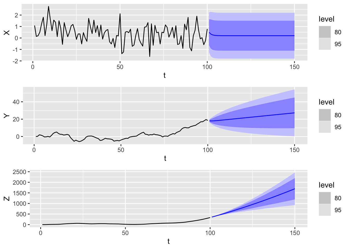
We generate sample trajectories and forecasts from the following three models: \[
(I- 0.5B)X_t = 0.1 + + W_t
\]\[
(I - 0.5B)(I-B)Y_t = 0.1 + W_t
\]\[
(I - 0.5B)(I-B)^2Z_t = 0.1 + W_t
\]
We use the same white noise process to create all three trajectories, so the sequence \((Y_t)\) is the discrete integral of \((X_t)\), and likewise, \((Z_t)\) is the discrete integral of \((Y_t)\).
Warning: Model specification induces a quadratic or higher order polynomial trend.
This is generally discouraged, consider removing the constant or reducing the number of differences.
grid.arrange(plt1, plt2, plt3, nrow =3)
Figure 12.1: Sample trajectories and forecasts for ARIMA(1,d,0) models with d = 0 (top), d = 1 (middle), and d = 2 (bottom) respectively.
Notice how the shape of the forecast curves depend on \(d\):
If \(d = 0\), then it converges to the mean \(\mu = 0.2\).
If \(d = 1\), then it converges to a straight line with slope \(\mu\).
If \(d = 2\), then it converges to a quadratic with curvature \(\mu\).
Moreover, for \(d > 1\), the width of the prediction intervals grows as \(h\) increases. Bear in mind the y-axis scale of the plots. Finally, we see that the trajectories become smoother as \(d\) increases.
12.4 Testing for stationarity
12.4.1 Unit roots and stationarity
As with the hyperparmeters \(p\) and \(q\), one has to estimate the appropriate order of differencing, \(d\), from data. Just as there are dangers with setting \(p\) and \(q\) to be unnecessarily large, we also do not want to difference too much. First, as seen in the previous section, this may lead to forecasts that are so uncertain as to be practically useless. Second, an overly differenced time series may develop undesirable properties. For instance, consider the \(\textnormal{AR}(1)\) model \[
X_t = \phi X_{t-1} + W_t.
\tag{12.10}\] If \(|\phi| < 1\), then taking a first difference gives \[
(I-B)X_t = \phi \cdot (I-B)X_{t-1} + W_t - W_{t-1}.
\] This makes \((I-B)X_t\) an \(\textnormal{ARMA}(1,1)\) model that is non-invertible.
As such, we want to be able to tell when differencing is needed and when it is not needed. This decision is best framed under an assumption that \((X_t)\) follows a (possibly non-causal or non-stationary) \(\textnormal{AR}(p)\) model, in which case, it is wholly dependent on whether the autoregressive polynomial \(\phi(z)\) has a root at \(z=1\). Such a root is called a unit root.
Suppose \(\phi(z)\) has a unit root and suppose it has multiplicity \(d\). Then we may factor it as \(\phi(z) = (1-z)^d\zeta(z)\) for some polynomial \(\zeta(z)\) without a unit root. In this case, the \(\textnormal{AR}(p)\) equation becomes \[
\zeta(B)(I-B)^dX_t = W_t,
\] and we see that \((I-B)^dX_t\) is stationary so long as all remaining roots of \(\zeta(z)\) lie outside the unit disc.
Conversely, if \(\phi(z)\) does not have a unit root, then the difference \((I-B)X_t\) satisfies a non-invertible \(\textnormal{ARMA}(p-1,1)\) model, just as in the \(\textnormal{AR}(1)\) case.
In summary, while a unit root is a sufficient but not necessary condition of being non-stationary, it is precisely the type of non-stationarity that can be fixed via differencing. We therefore introduce two unit root tests, i.e. tests for whether \(\phi(z)\) has a unit root.
12.4.2 The Dickey-Fuller (DF) test
The Dickey-Fuller test starts with assuming that the generating model is \(\textnormal{AR}(1)\). It then seeks to test the following null and alternate hypotheses:
To do this, we modify the equation to read \[
(I-B) X_t = (\phi-1)X_{t-1} + W_t.
\] Regressing \((I-B) X_t\) on \(X_{t-1}\) gives us an estimate for \(\phi - 1\). In the standard linear regression setting, the \(t\)-test is often used to test for a nonzero coefficient. However, such a test is not valid in this situation because of dependencies between the samples. Instead, we directly consider the rescaled fitted coefficient: \[
n (\hat \phi - 1) = \frac{n\sum_{t=1}^n (X_t - X_{t-1})X_{t-1}}{\sum_{t=1}^n X_{t-1}^2}
\tag{12.11}\] where by convention \(X_0 = 0\). This is called the Dickey-Fuller test statistic.
To obtain \(p\)-values from the test statistic, we need to know its (limiting) distribution under the null hypothesis. This is provided by the following proposition.
Proposition 12.3.(Limit of DF test statistic) Under \(H_0\), we have \[
n(\hat\phi - 1) \to_d \frac{\frac{1}{2}(W(1)^2 - 1)}{\int_0^1 W(t)^2dt},
\] where \(W(t)\) is a standard Brownian motion process.
A continuous time process \((W(t))_{t\geq 0}\) is called standard Brownian motion process if it satisfies
\(W(0) = 0\);
\(W(t_2) - W(t_1), W(t_3) - W(t_2),\ldots,W(t_n) - W(t_{n-1})\) are independent for any \(0 \leq t_1 < t_2 < \cdots <t_n\);
\(W(t+\Delta t) - W(t) \sim \mathcal N(0,\Delta t)\) for any \(\Delta t > 0\).
Proof (optional). First, rewrite Equation 12.11 as \[
\frac{\frac{1}{n\sigma^2}\sum_{t=1}^n (X_t - X_{t-1})X_{t-1}}{\frac{1}{n}\sum_{t=1}^n (\sigma^{-1}n^{-1/2}X_{t-1})^2}.
\] Under the null hypothesis, we have \(X_t = X_{t-1} + W_t\). Square both sides to get \[
X_t^2 = X_{t-1}^2 + 2X_{t-1}W_t + W_t^2.
\] Rearranging gives \[
2(X_t - X_{t-1})X_{t-1} = 2W_t X_{t-1} = X_t^2 - X_{t-1}^2 - W_t^2.
\] Summing up these terms for \(t=1,\ldots,n\) gives a telescoping sum, which allows us to rewrite the numerator of Equation 12.11 as \[
\frac{1}{n\sigma^2}\sum_{t=1}^n (X_t - X_{t-1})X_{t-1} = \frac{1}{2}\left(\frac{X_n^2}{n\sigma^2} - \frac{\sum_{t=1}^n W_t^2}{n\sigma^2}\right).
\] The second quantity converges to 1 in probability via the law of large numbers, while \[
\frac{X_n}{\sigma\sqrt n} = \frac{1}{\sigma\sqrt n}\sum_{t=1}^n W_t \to_d \mathcal{N}(0,1).
\] Using Slutsky’s theorem, we get \[
\frac{X_n^2}{n\sigma^2} - \frac{\sum_{t=1}^n W_t^2}{n\sigma^2} \to_d W(1)^2 - 1.
\] For the denominator, first notice that for a fixed constant \(0 < c < 1\), we have \[
\frac{1}{\sigma\sqrt n}X_{\lfloor cn \rfloor} \to_d \mathcal N(0,c)
\] by the regular central limit theorem (CLT). There exists a functional version of the CLT, which says that the random function \(c \mapsto \frac{1}{\sigma\sqrt n}X_{\lfloor cn \rfloor}\) converges in distribution to standard Brownian motion \(c \mapsto W(c)\). Using this, we get \[
\frac{1}{n}\sum_{t=1}^n (\sigma^{-1}n^{-1/2}X_{t-1})^2 \to_d \int_0^1 W(t)^2 dt.
\] Note that the distributions of the numerator and denominator jointly converge to their limits. By the continuous mapping theorem, the limit of the ratio has the desired distribution. \(\Box\)
Note
Note that the Dickey-Fuller is not valid if \((X_t)\) is not drawn from an \(\textnormal{AR}(1)\) model. There are versions of the test that relax this to accommodate mean and trend terms in the model.
12.4.3 The Augmented Dickey-Fuller (ADF) test
The ADF test modifies the DF test so that it is valid whenever \((X_t)\) is drawn from an \(\textnormal{AR}(p)\) model: \[
X_t = \sum_{j=1}^p \phi_j X_{t-j} + W_t.
\tag{12.12}\]
To obtain a test statistic, subtract \(X_{t-1}\) from both sides of Equation 12.12 to get \[
(I-B) X_t = \gamma X_{t-1} + \sum_{j=1}^{p-1} \psi_j (I-B) X_{t-j} + W_t,
\] where \(\gamma = \sum_{j=1}^p \phi_j - 1\), and \(\psi_j = - \sum_{i=j+1}^p \phi_i\) for \(j=1,\ldots,p-1\). Since \[
\gamma = \sum_{j=1}^p \phi_j - 1 = -\phi(1),
\]\(\phi\) has a unit root iff \(\gamma = 0\) and we seek to test the hypothesis \[
H_0: \gamma = 0.
\] This time the test statistic is the Wald statistic \(\frac{\hat\gamma}{se(\hat\gamma)}\). The limiting distribution is different, but is derived in a similar manner as in the case of Dickey-Fuller.
Note
Just like with the DF test, there are versions of the ADF test that can accommodate mean and trend terms in the model.
Although the ADF test assumes that an \(\textnormal{AR}(p)\) model, this assumption is relatively reasonable. We have already seen that any invertible \(\textnormal{ARMA}(p, q)\) model has an \(\textnormal{AR}(\infty)\) representation, and so can be approximated by \(\textnormal{AR}(p)\) so long as take \(p\) large enough.
Nevertheless, the ADF test requires us to choose what \(p\) to use for the null distribution. In practice, one rarely has a good a priori sense of what \(p\) should be, so one should choose \(p\) large enough so that enough of the lagged correlations are explained, but not so big that small numbers of samples for the larger lags cause instability. The function adf.test in tseries uses a default choice of \(p = n^{1/3}\). This also seems to be the choice also recommended by Said and Dickey (1984).
Note
The Phillips-Perron test is another popular unit root test that is similar to the ADF test. It is implemented using the function pp.test in tseries.
12.4.4 The KPSS test
One issue with the DF and ADF tests is that the null hypothesis is the presence of a unit root. In statistical hypothesis testing, there is an asymmetry between the null and alternate hypotheses: The null is only rejected when there is strong evidence against this. As such, if we difference a process if DF or ADF fail to reject, we will be especially aggressive and choose to do so even in cases where it doesn’t clearly help.
Due to this, Kwiatkowski, Phillips, Schmidt and Shin proposed a new test that used stationarity as the null hypothesis (see Kwiatkowski et al. (1992)). It assumes the generating distribution \[
X_t = R_t + Y_t
\tag{12.13}\] where \(Y_t\) is a stationary process and \(R_t\) is a random walk. In other words, \[
R_t = R_{t-1} + W_t
\] with \((W_t) \sim WN(0,\sigma^2)\), and \(R_0\) is a potentially nonzero offset term. We set the null and alternate hypothesis to be \[
H_0 : \sigma^2 = 0 \quad\quad\text{versus} \quad\quad H_1 : \sigma^2 > 0.
\] The null is equivalent to Equation 12.13 being stationary. Let \(S_t = \sum_{j=1}^t (X_j - \bar X)\) denote the partial sums of the centered process. The KPSS test statistic is \[
\frac{\sum_{t=1}^n S_t^2}{n^2 \hat V},
\] where \(\hat V\) is an estimate for \(V = \Var\left\lbrace S_n/\sqrt n\right\rbrace\).
Proposition 12.4. Suppose \(\hat V\) is a consistent estimator. Under \(H_0\), we have \[
\frac{\sum_{t=1}^n S_t^2}{n^2 \hat V} \to_d \int_0^1 B(t)^2 dt,
\] where \(B(t) \coloneqq W(t) - tW(1)\) is a Brownian bridge.
Proof (optional). Note that \(S_0 = 0\) and \(S_n = \sum_{j=1}^n X_j - n\bar X = 0\). By a functional central limit theorem (Herrndorf (1984)), the random function \[
c \mapsto \frac{S_{\lfloor c n \rfloor}}{\sqrt {n V}}
\] converges in distribution to a Brownian bridge \(c \mapsto B(c)\). Now combine this together with consistency for \(\hat V\) and use Slutsky’s theorem. \(\Box\)
Using Theorm 9.1, \[
V = \sum_{h=-n}^n \left(1 - \frac{|h|}{n}\right)\gamma_X(h).
\] A consistent estimator is given by3\[
\hat V = \sum_{h=-\sqrt n}^{\sqrt n} \left( 1 - \frac{|h|}{\sqrt n}\right)\hat \gamma_X(h).
\]
Note
Just as in the ADF test, we can modify the test to include a linear trend in the null hypothesis.
12.4.5 Unit root tests in R
Unit tests in R can be computed using functions from the tseries package. The ADF test can be computed using adf.test, while the KPSS test can be computed using kpss.test. Note that adf.test automatically includes a trend and constant term, i.e. the null model is \[
\phi(B)X_t = \alpha + \beta t + W_t,
\] where \(\phi(B)\) has a unit root. The KPSS test also automatically includes these terms by default, but has an option to select otherwise.
We illustrate their use for the sunspots data introduced in Chapter 10.
Warning in adf.test(sunspots$Sunspots): p-value smaller than printed p-value
    Augmented Dickey-Fuller Test

data:  sunspots$Sunspots
Dickey-Fuller = -5.3313, Lag order = 6, p-value = 0.01
alternative hypothesis: stationary
sunspots$Sunspots |>kpss.test()
Warning in kpss.test(sunspots$Sunspots): p-value greater than printed p-value
    KPSS Test for Level Stationarity

data:  sunspots$Sunspots
KPSS Level = 0.20311, Truncation lag parameter = 5, p-value = 0.1
Note that both tests produce warnings about their p-values. This is because the printed p-values are computed by interpolating values from a table. With this caveat, the ADF test produces a p-value of at most 0.01, which provides evidence to reject the existence of a unit root. Meanwhile, the KPSS test produces a p-value of at least 0.1, which means that there is insufficient evidence to reject the null hypothesis that the time series is stationary.
The feasts package allows us to compute these tests efficiently at scale.
# A tibble: 8 × 6
  Animal State                        kpss_stat kpss_pvalue ndiffs nsdiffs
  <fct>  <fct>                            <dbl>       <dbl>  <int>   <int>
1 Calves Australian Capital Territory    3.62          0.01      1       0
2 Calves New South Wales                 3.10          0.01      1       0
3 Calves Northern Territory              2.21          0.01      1       0
4 Calves Queensland                      5.75          0.01      1       0
5 Calves South Australia                 6.08          0.01      1       0
6 Calves Tasmania                        0.0890        0.1       0       1
7 Calves Victoria                        2.04          0.01      1       1
8 Calves Western Australia               4.21          0.01      1       0
Note that aus_livestock is a quarterly time series dataset recording the number of each type of livestock animal in Australia, stratified by state. Here, we focus on the time series measuring the number of calves and have computed the KPSS test statistic and p-value. unitroot_ndiffs calculates the appropriate number of first differences based on this value, while unitroot_nsdiffs calculates the appropriate number of seasonal differences based on the “strength of seasonality” statistic.
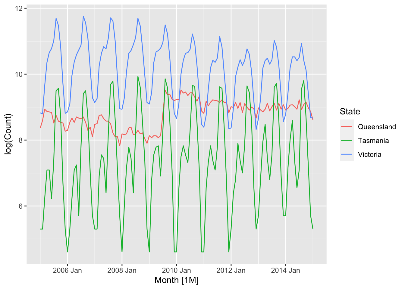
Let us do a time plot to get further intuition for these numbers. For ease of interpretation, we only plot values between January 2005 and January 2015 and for the log counts in 3 states: Queensland, Tasmania, and Victoria.
Figure 12.2: The log counts of the number of calves in Queensland, Tasmania and Victoria.
We see that the Queensland time series does not have any seasonality but has a non-stationary level. Next, the Tasmania time series has non-stationary seasonality but its level seems stationary. Finally, the Victoria time series has both non-stationary seasonality as well as a non-stationary level.
12.5 ARIMA modeling with fable
12.5.1 Function syntax
The general recipe for fitting ARIMA models in fable is to write
ARIMA(X ~pdq(p, d, q) +PDQ(P, D, Q, period = m) + k)
The various components of this snippet have the following meanings:
X: column name of the time series being modeled
p: the non-seasonal autoregressive order
q: the non-seasonal moving average order
d: the order of non-seasonal differencing
P: the seasonal autoregressive order
Q: the seasonal moving average order
D: the order of seasonal differencing
m: the period of the seasonality
k: \(1\) if a mean parameter is to be fit, \(0\) otherwise
If any hyperparameter is not specified, it is automatically estimated from the data. One may also choose to provide a range of possible values for each hyperparameter instead of allowing the code to search over all possibilities. We refer the reader to the function documentation for more details on its useage.
12.5.2 Model selection
Model selection is performed using a version of the Hyndman-Khandakar algorithm (Hyndman and Khandakar (2008)). The algorithm comprises of two steps:
Step 1. Determine the order of differencing \(d\) (and \(D\)) by performing repeated KPSS tests.
Step 2. Do a local search over \(p\), \(q\), \(P\), \(Q\), and \(k\) (within the specified constraints). For each iteration, we compare the AICc value of the current model with those of models fitted with adjacent hyperparameter values (e.g. with \((p', q, P, Q, k)\) such that \(p' = p \pm 1\)). Stop when a local minimum is found.
Caution
We cannot use AICc to compare models with different values of differencing. This is because the likelihood functions at different levels of differencing have different meanings and are incomparable. In other words, doing so is similar to comparing two different models, but evaluating each with a different loss function. For the same reason, we cannot use AICc to compare a pair of models in which only one of them is applied with a transformation (e.g. a log transform.)
12.6 Data examples
12.6.1 Sunspots
Let us apply ARIMA modeling to the sunspot data from Chapter 10. We shall simultaneously fit an \(\textnormal{AR}(2)\) model as before as well as let ARIMA() perform an automatic search.
# A mable: 1 x 2
                     ar2                 search
                 <model>                <model>
1 <ARIMA(2,0,0) w/ mean> <ARIMA(2,0,1) w/ mean>
We see that ARIMA() has returned an \(\textnormal{ARMA}(2, 1)\) model with a mean term. We can inspect the log likelihood, AIC, and AICc values for each of these models by calling glance():
# A tibble: 2 × 3
  .model  MASE RMSSE
  <chr>  <dbl> <dbl>
1 ar2    0.875 0.850
2 search 0.881 0.847
Here, we see that the comparison is a bit ambiguous. Finally, we perform a residual analysis to check whether the model is a good fit.
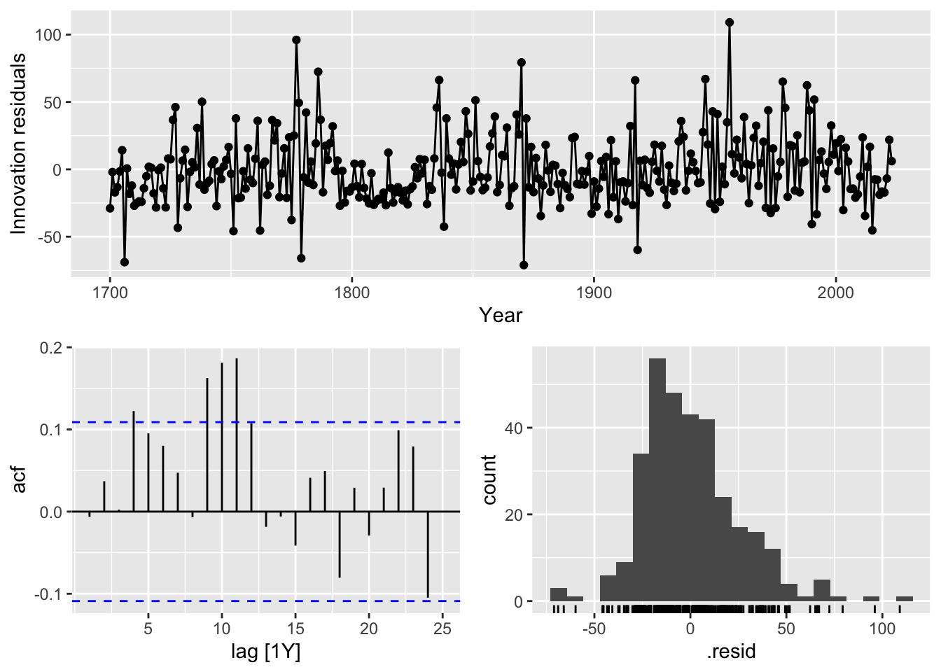
sunspots_fit |>select(search) |>gg_tsresiduals()
The ACF plot shows that there are some residual autocorrelations, which means that the model is not a very good fit. The residual density plot shows that there is some skewness in favor of positive residuals, which implies that a Box-Cox transformation might be appropriate.
12.6.2 Tourist arrivals
We now fit ARIMA and exponential smoothing models to the Australian tourist arrivals dataset.
# A mable: 1 x 3
# Key:     Origin [1]
  Origin                    arima          ets
  <chr>                   <model>      <model>
1 Japan  <ARIMA(0,1,1)(1,1,1)[4]> <ETS(M,A,M)>
Here, we see that ARIMA() selects a seasonal \(\textnormal{ARIMA}(0, 1, 1)(1, 1, 1)_4\) model, while ETS() fits a Holt-Winters model with multiplicative noise and seasonality.
# A tibble: 2 × 3
  .model  MASE RMSSE
  <chr>  <dbl> <dbl>
1 arima   1.03 0.990
2 ets     1.06 1.07
Performing cross-validation, we see that the ARIMA model performs slightly better with a forecast horizon of \(h = 5\).
Brockwell, Peter J, and Richard A Davis. 1991. Time Series: Theory and Methods. Springer science & business media.
Herrndorf, Norbert. 1984. “A Functional Central Limit Theorem for Weakly Dependent Sequences of Random Variables.”The Annals of Probability, 141–53.
Hyndman, Rob J, and George Athanasopoulos. 2018. Forecasting: Principles and Practice. OTexts.
Hyndman, Rob J, and Yeasmin Khandakar. 2008. “Automatic Time Series Forecasting: The Forecast Package for r.”Journal of Statistical Software 27: 1–22.
Kwiatkowski, Denis, Peter CB Phillips, Peter Schmidt, and Yongcheol Shin. 1992. “Testing the Null Hypothesis of Stationarity Against the Alternative of a Unit Root: How Sure Are We That Economic Time Series Have a Unit Root?”Journal of Econometrics 54 (1-3): 159–78.
Said, Said E, and David A Dickey. 1984. “Testing for Unit Roots in Autoregressive-Moving Average Models of Unknown Order.”Biometrika 71 (3): 599–607.
This further supports our interpretation of differencing as discrete differentiation.↩︎
Another way to see this is to use the expansion \(\frac{1}{(1-x)^n} = \frac{1}{n}\frac{d^{n-1}}{dx^{n-1}}\frac{1}{1-x}\). The coefficient of the \(k\)-th term is then \(\frac{(k+1)(k+2)\cdots(k+n-1)}{(n-1)!}\).↩︎