10  Autoregressive Models

10.1 Motivation

10.1.1 Sunspot data

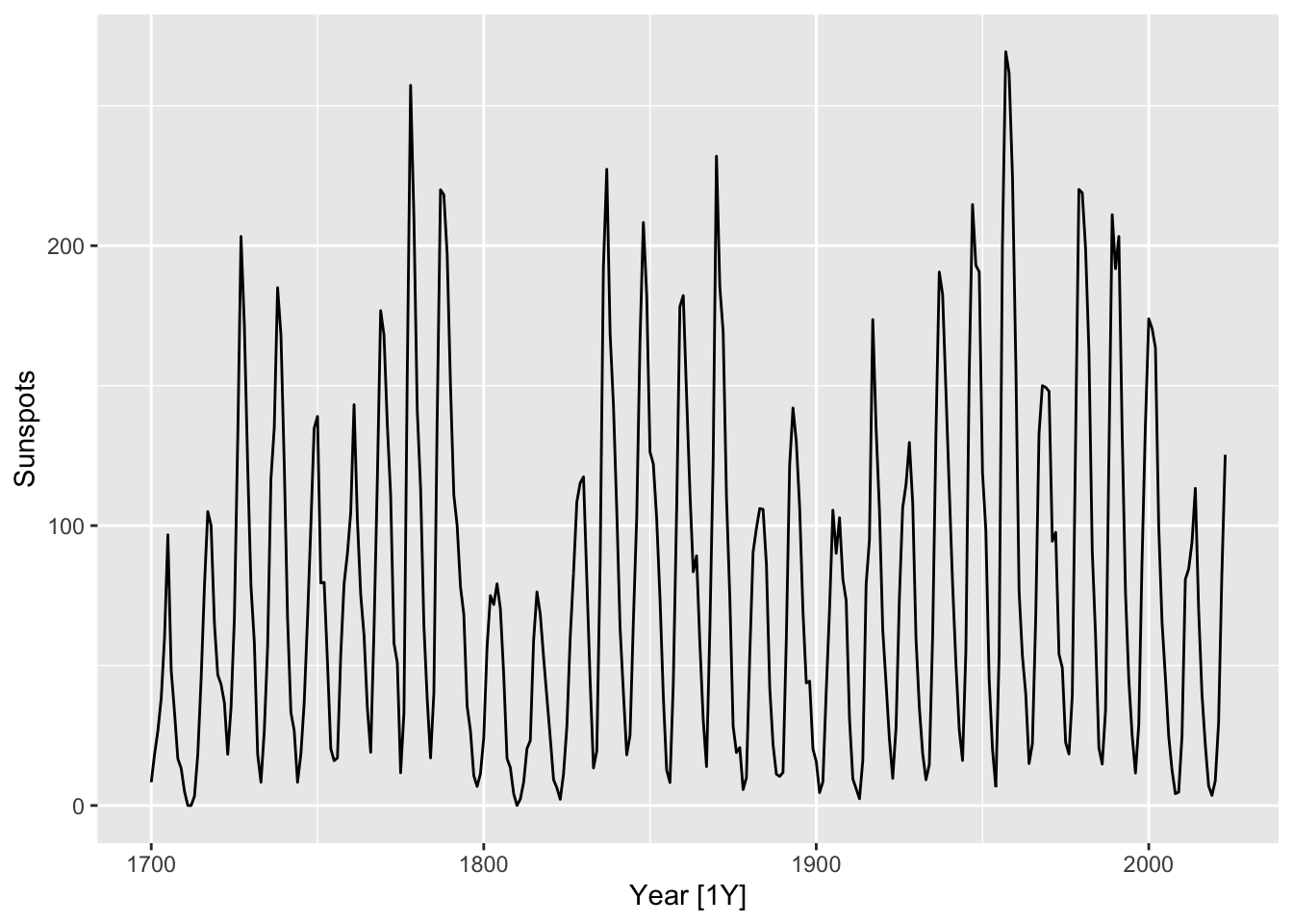
Sunspots are regions of the Sun’s surface that appear temporarily darker than the surrounding areas. They have been studied by astronomers since ancient times, and their frequency is known to have approximately periodic behavior, with a period of about 11 years. In the following figure, we plot the mean daily total sunspot number for each year between 1700 and 2023.

sunspots <- read_rds("_data/cleaned/sunspots.rds")
sunspots |> autoplot(Sunspots)

Figure 10.1: Yearly mean total sunspot number obtained by taking a simple arithmetic mean of the daily total sunspot number over all days of each year.

10.1.2 A sinusoidal model

In view of the data’s periodic nature, it seems to make sense to fit a signal plus noise model of the form \[ X_t = \mu + \alpha_1 \cos(\omega t) + \alpha_2 \sin(\omega t) + W_t, \tag{10.1}\] where \(\omega = 2\pi/11\) and \((W_t) \sim WN(0,\sigma^2)\) for an unknown \(\sigma^2\) parameter to be estimated.

sunspots_fit <- sunspots |>
    model(sin_model = TSLM(Sunspots ~ sin(2 * pi * Year / 11) + 
                           cos(2 * pi * Year / 11)))
sigma <- sunspots_fit |>
    pluck(1, 1, "fit", "sigma2") |>
    sqrt()

We next plot the fitted values for the model together with a draw of a sample trajectory generated from the model. We also make plots of its residual diagnostics.

Fitted values

set.seed(5209)
sunspots_fit |>
    augment() |> 
    mutate(Sample = .fitted + rnorm(nrow(sunspots)) * sigma,
           Observed = sunspots$Sunspots) |>
    rename(Fitted = .fitted) |>
    pivot_longer(cols = c("Fitted", "Observed", "Sample"),
                 values_to = "Number",
                 names_to = "Type") |>
    filter(Year > 1900) |>
    ggplot() +
    geom_line(aes(x = Year, y = Number, color = Type)) + 
    scale_color_manual(values = c("Fitted" = "blue", "Observed" = "black", "Sample" = "orange"))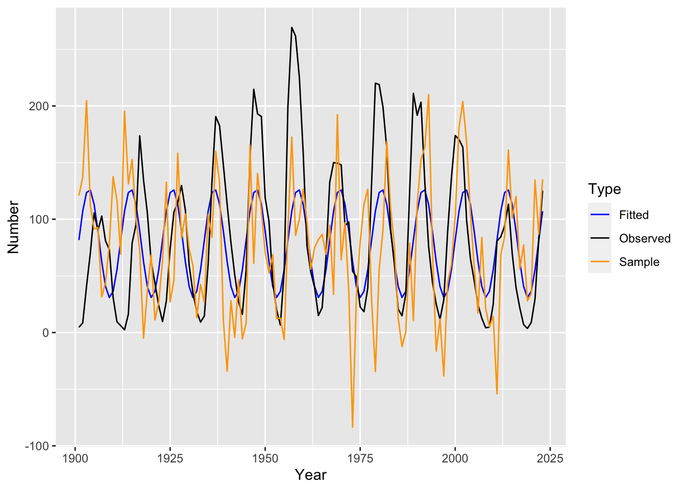

Figure 10.2: Yearly mean daily total sunspot number (black), the mean function of a sinusoidal signal plus noise model fitted to the data (blue), and a sample trajectory from the model (orange).

Residuals

sunspots_fit |>
    gg_tsresiduals()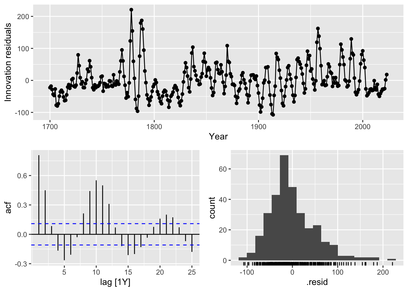

Figure 10.3: Residual diagnostics for the signal plus noise model for yearly mean daily total sunspot number.

We see that the model residuals do not look like white noise, implying that the model has a poor fit. More precisely, inspecting the fitted values, we observe the following issues:

• Some of the observed oscillations (e.g. around 1960) have much higher amplitude than can be explained by a single sinusoid.
• The period of the oscillation is not fixed but varies slightly over time.
• The sample trajectory seems much more noisy than the observed time series.

For this reason, Udny Yule proposed an alternative model that is also based on a single sinusoid, but which incorporates noise in a different way.

10.1.3 Periodic behavior from ODEs

Yule’s starting observation was the fact that the mean function of Equation 10.1, \[ x(t) = \mu + \alpha_1 \cos(\omega t) + \alpha_2 \sin(\omega t), \tag{10.2}\] is a solution to the ordinary differential equation (ODE) \[ x''(t) = - \omega^2 \left(x(t) - \mu\right). \tag{10.3}\] Indeed, ODE theory tells us that all solutions to this ODE are of the form Equation 10.2 for some choice of \(\alpha_1\) and \(\alpha_2\) determined by initial conditions.

An ODE tells us how a physical system evolves deterministically based on its inherent properties. For instance, Equation 10.3 is also the ODE governing the small angle oscillation of a pendulum resulting from gravity, which means that the pendulum’s angular position is given by Equation 10.2. The periodic nature of the sunspot data is suggestive of a similar mechanism at work. On the other hand, the departures from pure periodicity suggests that this evolution is not determinstic, but is affected by external noise (which may comprise transient astrophysical phenomena).¹ In order to accommodate this, we can add a noise term into Equation 10.3 to get a stochastic differential equation: \[ d^2X_t = - \omega^2 \left(X_t - \mu\right) + dW_t. \] Since time series deals with discrete time points, however, we will first re-interpret Equation 10.3 in a discrete setting.

Note

As seen above, stochastic differential equations are natural generalizations of ODEs, and are used to model complex dynamical systems arising in finance, astrophysics, biology, and other fields. They are beyond the scope of this textbook.

10.1.4 Periodic behavior from difference equations

The discrete time analogue of an ODE is a difference equation, which relates the value of a sequence at time \(t\) to its values at previous time points.

Proposition 10.1. The time series Equation 10.2 is the unique general solution to the difference equation: \[ (I-B)^2 x_t = 2(\cos \omega - 1)(x_{t-1} - \mu). \tag{10.4}\]

Here, \(B\) is the backshift operator defined in Chapter 4. Observe the similarity between Equation 10.3 and Equation 10.4, especially bearing in mind that the difference operator \(I-B\) can be thought of as discrete differentiation.

10.1.5 An autoregressive model

Following the argument in Section 10.1.3, Yule (1927) proposed the model: \[ (I-B)^2 X_t = 2(\cos \omega - 1)(X_{t-1} - \mu) + W_t, \tag{10.5}\] where \((W_t) \sim WN(0,\sigma^2)\). The parameters to be estimated are \(\omega\), \(\mu\), and \(\sigma^2\). In other words, at each time point, the second derivative is perturbed by an amount of exogenous (external) noise.

Note that Equation 10.5 can be rewritten as \[ X_t = \alpha + 2\cos \omega X_{t-1} - X_{t-2} + W_t, \] with \(\alpha = 2(1-\cos\omega)\mu\). In other words, \(X_t\) is a linear combination of its previous two values together with additive noise. It is an example of an autoregressive model of order 2, which we will soon formally define.

We now fit the model and plot both its one-step ahead fitted values \(\hat X_{t|t-1}\) as well as a sample trajectory generated from the model. As before, we also make plots of its residual diagnostics.

sunspots_fit <- sunspots |>
    model(ar_model = AR(Sunspots ~ order(2)))
sigma <- sunspots_fit |>
    pluck(1, 1, "fit", "sigma2") |>
    sqrt()

Fitted values

set.seed(5209)
sunspots_fit |>
    augment() |> 
    mutate(Sample = sim_ar(sunspots_fit),
           Observed = sunspots$Sunspots) |>
    rename(Fitted = .fitted) |>
    pivot_longer(cols = c("Fitted", "Observed", "Sample"),
                 values_to = "Number",
                 names_to = "Type") |>
    filter(Year > 1900) |>
    ggplot() +
    geom_line(aes(x = Year, y = Number, color = Type)) + 
    scale_color_manual(values = c("Fitted" = "blue", "Observed" = "black", "Sample" = "orange"))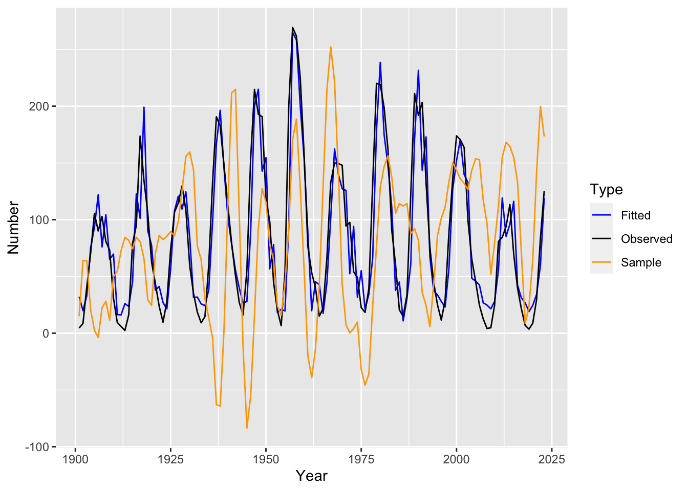

Figure 10.4: Yearly mean daily total sunspot number (black), the one-step ahead fitted values using Yule’s fitted model (blue), and a sample trajectory from the model (orange).

Residuals

sunspots_fit |>
    gg_tsresiduals()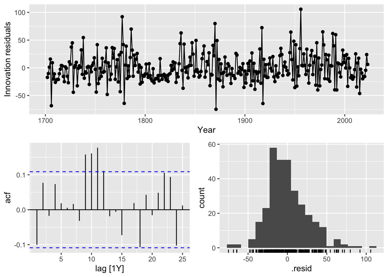

Figure 10.5: Residual diagnostics for Yule’s model for yearly mean daily total sunspot number.

We see that the residuals look much closer to white noise than those of the signal plus noise model, although there still seems to be some remaining outlier values as well as periodic behavior. Furthermore, the fitted values are much closer to the observed time series, and a sample trajectory from the model now seems qualitatively similar to the observed time series (apart from the negative values).

10.1.6 Final comparison

We have seen that Yule’s model gives a much better fit to the data than the signal plus noise model. As a final comparison between the two models, observe that we can rewrite each model as a pair of equations. First, using Proposition 10.1, the signal plus noise model is equivalent to the following: \[ (I-B)^2 Y_t = 2(\cos \omega - 1)(Y_{t-1} - \mu) \] \[ X_t = Y_t + W_t. \] Meanwhile, Yule’s model is trivially equivalent to: \[ (I-B)^2 Y_t = 2(\cos \omega - 1)(Y_{t-1} - \mu) + W_t \] \[ X_t = Y_t. \]

In both cases, we can think of \(Y_t\) as defining the true state of nature at time \(t\), whose values directly affect its future states. Meanwhile, \(X_t\) reflects our observation of the state of nature at time \(t\). The signal plus noise model postulates a deterministic evolution of the true state, but introduces observational noise. On the other hand, Yule’s model postulates noiseless observations, but allows for a noisy evolution of the state of nature. It is possible to incorporate both sources of noise in the same model. We will discuss this further when we cover state space models.

10.2 Introducing AR models

An autoregressive model of order \(p\), abbreviated \(\textnormal{AR}(p)\), is a stationary stochastic process \((X_t)\) that solves the equation \[ X_t = \alpha + \phi_1 X_{t-1} + \phi_2 X_{t-2} + \cdots + \phi_p X_{t-p} + W_t, \tag{10.6}\] where \((W_t) \sim WN(0,\sigma^2)\), and \(\phi_1, \phi_2,\ldots,\phi_p\) are constant coefficients.

It is similar to a regression model, except that the regressors are copies of the same time series variable, albeit at earlier time points, hence the term autoregressive.

Note that a simple rearrangement of Equation 10.6 shows that it is equivalent to \[ X_t - \mu = \phi_1 (X_{t-1} - \mu) + \phi_2 (X_{t-2} - \mu) + \cdots + \phi_p (X_{t-p} - \mu) + W_t, \] where \(\mu = \alpha/(1- \phi_1 - \phi_2 - \cdots \phi_p)\). We will soon see that this implies that the mean of \((X_t)\) is \(\mu\). It also implies that centering an autoregressive model does not change its coefficients.

The autoregressive polynomial of the model Equation 10.6 is \[ \phi(z) = 1 - \phi_1 z - \phi_2 z^2 - \cdots - \phi_p z^p. \] Using this notation, we can rewrite Equation 10.6 as \[ \phi(B)(X_t - \mu) = W_t, \] where \(B\) is the backshift operator. We call \(\phi(B)\) the autoregressive operator. Note that for any integer \(k\), \(B^k\) is the composition of the backshift operator \(B\) with itself \(k\) times. Since \(B\) shifts the sequence forwards by one time unit, this resulting operator therefore shifts a sequence forwards by \(k\) time units.

Note

More formally, we can regard \(B\) as an operator on the space of doubly infinite sequences \(\ell^\infty(\Z)\). In other words, it is a linear mapping from \(\ell^\infty(\Z)\) to itself. Mathematically, we say that the space of operators form an algebra. Operators can be added and multiplied like vectors: The resulting operator just outputs the sum or scalar multiple of the original outputs. They can also be composed as discussed earlier.

Introducing this formalism turns out to be quite useful. Apart from allowing for compact notation, the properties of the autoregressive polynomial \(\phi\), in particular its roots and inverses, turn out to be intimately related to properties of the \(\textnormal{AR}(p)\) model.

It is important to understand that Equation 10.6 and its variants are equations and that the model is defined as a solution to the equation. A priori, such a solution may not exist at all, or there may be multiple solutions.

10.3 AR(1)

We illustrate some of the basic properties of autoregressive models by studying its simplest version, \(\textnormal{AR}(1)\). This is defined via the equation \[ X_t = \phi X_{t-1} + W_t, \tag{10.7}\] where \((W_t) \sim WN(0,\sigma^2)\).² It is convention to slightly abuse notation, using \(\phi\) to denote both the AR polynomial and its coefficient. The meaning will be clear from the context.

10.3.1 Causal solutions

Proposition 10.2 (Existence and uniqueness of solutions). Suppose \(|\phi| < 1\), then there is a unique stationary solution to Equation 10.7. This solution is a causal linear process.

Proof. We first show existence. Consider the random variable defined as \[ X_t \coloneqq \sum_{j=0}^\infty \phi^j W_{t-j}. \tag{10.8}\] Since \[ \sum_{j=0}^\infty |\phi^j| = \frac{1}{1-|\phi|} < \infty, \] the expression converges in a mean squared sense, so \(X_t\) is well-defined. Indeed, \((X_t)\) defined in this manner is a causal linear process and is in particular stationary. It is also easy to see that it satisfies Equation 10.7: \[ \begin{split} \phi X_{t-1} + W_t & = \phi\left(\sum_{j=0}^\infty \phi^j W_{t-1-j}\right) + W_t \\ & = \sum_{j=0}^\infty \phi^{j+1} W_{t-1-j} + W_t \\ & = \sum_{k=1}^\infty \phi^{k} W_{t-k} + W_t \\ & = X_t. \end{split} \]

To see that it is unique, suppose we have another stationary solution \((Y_t)\). We may then use Equation 10.7 to write \[ \begin{split} Y_t & = \phi Y_{t-1} + W_t \\ & = \sum_{j=0}^{l-1} \phi^j W_{t-j} + \phi^l Y_{t-l}, \end{split} \] where the second equality holds for any integer \(l > 0\). We thus see that for the same white noise sequence, we have \[ Y_t - X_t = -\sum_{j=l}^\infty \phi^j W_{t-j} + \phi^l Y_{t-l}. \] We can obtain a variance bound on the right hand side that tends to 0 as \(l \to \infty\): \[ \begin{split} \Var\left\lbrace -\sum_{j=l}^\infty \phi^j W_{t-j} + \phi^l Y_{t-l} \right\rbrace & \leq 2\Var\left\lbrace \sum_{j=l}^\infty \phi^j W_{t-j}\right\rbrace + 2\Var\left\lbrace \phi^l Y_{t-l}\right\rbrace \\ & = \frac{2\phi^{2l}\sigma^2}{1-\phi^2} + \phi^{2l}\gamma_Y(0). \end{split} \] Since the left hand side is independent of \(l\), we get \(Y_t =_d X_t\) as we wanted. \(\Box\)

This theorem allows us to speak of the solution to Equation 10.7, and we sometimes informally refer to the equation as the model. As such, we also refer to Equation 10.7 for \(|\phi| < 1\) as a causal \(\textnormal{AR}(1)\) model.

10.3.2 Moments

Proposition 10.3 (Mean, ACVF, ACF). Let \((X_t)\) be the solution to Equation 10.7. Then we have \(\mu_X = 0\) and \[ \gamma_X(h) = \frac{\sigma^2\phi^h}{1-\phi^2}, \] \[ \rho_X(h) = \phi^h \] for all positive integers \(h\).

Proof. Using Equation 10.8, we get \[ \mu_X = \E\left\lbrace \sum_{j=0}^\infty \phi^j W_{t-j} \right\rbrace = \sum_{j=0}^\infty \phi^j \E\left\lbrace W_{t-j} \right\rbrace = 0. \]

There are two methods for calculating the ACVF.

Method 1. Equation 9.4, we get \[ \gamma_X(h) = \sigma^2 \sum_{j=0}^\infty \phi^j \phi^{j+h} = \frac{\sigma^2\phi^h}{1-\phi^2}. \]

Method 2. Multiplying Equation 10.7 by \(X_{t-h}\), we get \[ X_tX_{t-h} = \phi X_{t-1}X_{t-h} + W_tX_{t-h} \] and taking expectations gives \[ \gamma_X(h) = \begin{cases} \phi \gamma_X(1) + \sigma^2 & \text{if}~h = 0 \\ \phi\gamma_X(h-1) & \text{if}~h > 0. \end{cases} \] This yields the initial value \(\gamma_X(0) = \sigma^2/(1-\phi^2)\), and a recurrence relation (i.e. difference equation) that we may use to solve for the subsequent values. \(~\Box\)

In particular, we see that the ACF has an exponential decay.

10.3.3 Forecasts

The recurrence form of Equation 10.7 makes forecasting extremely straightforward. Recall that we are interested in both distributional and point forecasts (see Section 7.9). Given a statistical model and observations \(x_1,x_2,\ldots,x_n\) drawn from the model, the distributional forecast for a future observation \(X_{n+h}\) is just its conditional distribution given our observed values: \[ \P\left\lbrace X_{n+h} \leq x_{n+h}|X_1 = x_1, X_2 = x_2,\ldots,X_n = x_n \right\rbrace. \tag{10.9}\]

Given an \(\textnormal{AR}(1)\) model with a further assumption of Gaussian white noise, the distributional forecast is extremely easy to derive. We simply recursively apply Equation 10.7 to get \[ X_{n+h} = W_{n+h} + \phi W_{n+h-1} + \cdots + \phi^{h-1}W_{n+1} + \phi^hX_n. \] Since \(W_{n+1},\ldots,W_{n+h}\) are independent of \(X_1,X_2,\ldots,X_n\), this means that Equation 10.9 is simply \(N\left(\phi^h x_n, \frac{(1-\phi^{2h})\sigma^{2}}{1-\phi^2} \right)\). In particular, we get \[ \hat x_{n+h|n} = \phi^h x_n \] and a prediction interval at the 95% level is \[ (\phi^h x_n - 1.96v_h^{1/2} , \phi^h x_n + 1.96v_h^{1/2}), \] where \(v_h = \frac{(1-\phi^{2h})\sigma^{2}}{1-\phi^2}\).

Note that as the forecast horizon \(h\) increases, the point forecast converges to \(\mu_X = 0\), while the variance of the forecast distribution increases to \(\gamma_X(0) = \sigma^2/(1-\phi^2)\). In other words, the forecast distribution converges to the marginal distribution of \(X_t\) (for any \(t\)), and we see that our observations become increasingly irrelevant as we forecast further out into the future.

10.3.4 Sample trajectories

In the plot below, we create sample trajectories from \(\textnormal{AR}(1)\) models with \(\phi\) set to be \(0.3\), \(0.9\) and \(-0.9\) (from top to bottom). We also show the distributional forecasts up to the horizon \(h=20\).

Figure 10.6: Sample trajectories and forecasts for AR(1) models with different values of phi. These are (from top to bottom) 0.3, 0.9 and -0.9. The noise variance is set to be 1.

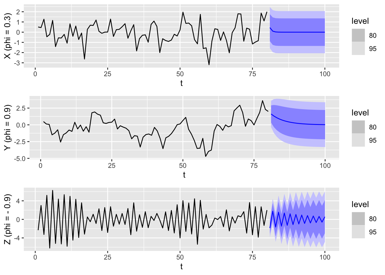
We see that \(\phi\) has a strong effect on both the shape of the trajectory as well as the forecasts. When \(\phi\) is small and positive, then the trajectory looks similar to that of white noise, whereas when \(\phi\) is large and positive, there are fewer fluctuations, and it looks similar to a random walk. The point forecasts also decay more slowly towards the mean. Finally, when \(\phi\) is negative, consecutive values are negatively correlated, which results in rapid fluctuations.

10.3.5 Reversibility and backcasts

If we assume that the white noise in Equation 10.7 is Gaussian, then the resulting \(\textnormal{AR}(1)\) process is also a Gaussian process, which means that its distribution is fully determined by its mean and ACVF functions. Note that the ACVF function of any stationary process is even: \(\gamma_X(h) = \gamma_X(-h)\). This means the covaraince matrix of \((X_1,X_2,\ldots,X_n)\), \(\Gamma_{1:n} = (\gamma_X(i-j))_{ij=1}^n\), is symmetric and so the distribution of \((X_1,X_2,\ldots,X_n)\) is the same as that of its time reversal \((X_n,X_{n-1},\ldots,X_1)\). In summary, stationary \(\textnormal{AR}(1)\) processes are reversible, and we cannot tell the direction of time simply by looking at a trajectory.

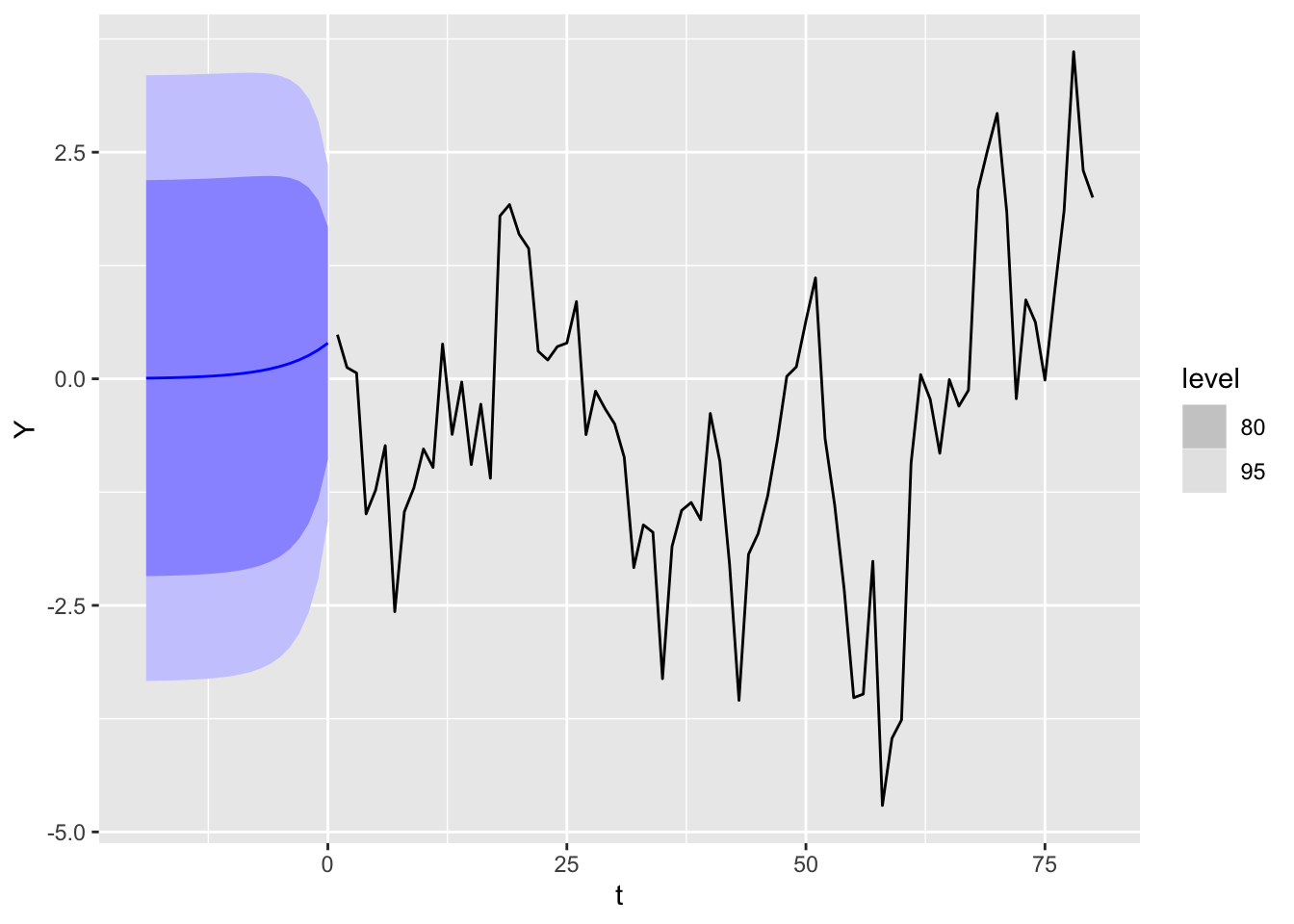
Many real world time series are not reversible, which means that \(\textnormal{AR}(1)\) models (and linear processes more generally) are poor fits whenever this holds. On the other hand, reversibility allows us to easily perform backcasting, which is the estimation of past values of a time series that are unknown.

Figure 10.7: Sample trajectory and backcasts for an AR(1) model with phi = 0.9.

10.3.6 Estimation

An \(\textnormal{AR}(1)\) model only has two parameters: \(\phi\) and \(\sigma^2\). Given observed data \(x_1,x_2,\ldots,x_n\), we may estimate these parameters as follows. First, Proposition 10.3 tells us that \(\phi = \rho_X(1)\), so we may use the estimator \(\hat\phi \coloneqq \hat\rho_X(1)\). Substituting this into Theorem 9.2 then gives \[ \sqrt n (\hat\phi - \phi) \to_d N(0,1-\phi^2). \]

Since \(\sigma^2 = \gamma_X(0)(1-\phi^2)\), we may estimate \[ \hat\sigma^2 \coloneqq \hat\gamma_X(0)(1 - \hat\rho_X(1)^2) = \hat\gamma_X(0) - \hat\gamma_X(1)^2/\hat\gamma_X(0). \] Since the sample ACVF is consistent (Theorem A.6 in Shumway and Stoffer (2000)), so is this estimator.

10.3.7 When \(|\phi| > 1\)

If a choice of \(|\phi| < 1\) results in a unique stationary solution, what happens when \(|\phi| > 1\)?

Explosive solution. If we start with a fixed initial value \(X_0 = c\), we can iterate Equation 10.7 to get \[ X_t = \sum_{j=0}^{t-1} \phi^j W_{t-j} + \phi^t c. \] The mean function is thus \(\mu_X(t) = \phi^t c\), while the marginal variance is given by \[ \gamma_X(t, t) = \Var\left\lbrace \sum_{j=0}^{t=1} \phi^j W_{t-j}\right\rbrace = \frac{\sigma^2(\phi^{2t}-1)}{\phi^2 - 1}. \] Both values diverge to infinity exponentially as \(t\) increases. The resulting time series model is sometimes called an explosive \(\textnormal{AR}(1)\) process. In particular, it is not stationary.

The above is probably unsurprising. When \(\phi = 1\), then Equation 10.7 is the defining equation for a random walk, which we already know is non-stationary. It is therefore somewhat unintuitive that there exist unique stationary solutions to Equation 10.7 when \(|\phi| > 1\).

Stationary solution. Define the expression \[ X_t \coloneqq -\sum_{j=1}^\infty \phi^{-j}W_{t+j}. \tag{10.10}\] Using the same arguments as in the proof of Proposition 10.2, one can check that this converges absolutely, and that \((X_t)\) is stationary and satisfies Equation 10.7. Indeed, it is the unique such solution. On the other hand, this solution doesn’t make physical sense because \(X_t\) depends on the future innovations \(W_{t+1}, W_{t+2},\ldots\).³ Formally, we say that such a solution is non-causal, unlike Equation 10.8.

Because of the the problems of these two solutions, Equation 10.7 with \(|\phi| > 1\) is rarely used for modeling.

Note

One may calculate the ACVF of Equation 10.10 to be \[ \gamma_X(h) = \frac{\sigma^2\phi^{-2}\phi^{-h}}{1-\phi^{-2}}. \] This is the same as that of a causal \(\textnormal{AR}(1)\) process with noise variance \(\tilde\sigma^2 \coloneqq \sigma^2\phi^{-2}\) and coefficient \(\tilde\phi \coloneqq \phi^{-1}\). If we assume Gaussian white noise, this implies that the two time series models are the same.

10.4 Causal solutions

We now generalize our findings about \(\textnormal{AR}(1)\) models to general \(\textnormal{AR}(p)\) models. Along the way, we will see that while the flavor of the results remains consistent, the technical difficulty of the tools we need increases sharply.

Theorem 10.4 (Existence and uniqueness of solutions) Let \(\phi(z)\) be the autoregressive polynomial of Equation 10.6. Suppose \(\phi(z) \neq 0\) for all \(|z| \leq 1\), then Equation 10.6 admits a unique stationary solution.⁴ This solution is causal and has the form \[ X_t = \mu + \sum_{j=0}^\infty \psi_j W_{t-j}, \tag{10.11}\] where \[ \phi(z) \cdot \left(\sum_{j=0}^\infty \psi_j z^j \right) = 1. \tag{10.12}\]

Note that by expanding out the product on the left hand side of Equation 10.12 and comparing coefficients of each monomial term with the right hand side, we get an infinite sequence of equations, which allows us to solve for \(\psi_0,\psi_1,\ldots\) (see Example 3.12 in Shumway and Stoffer (2000)).

Proof. The proof is slightly technical and boils down to investigating whether the autoregressive operator \(\phi(B)\) has a well-defined inverse. First, note that \(\phi(z)\) always has a formal power series inverse \(\sum_{j=0}^\infty \psi_j z^j\) obtained by solving Equation 10.12. To check its radius of convergence, write \(\phi(z) = \prod_{k=1}^r (1 - z_k^{-1}z)^{m_k}\), where \(z_1,z_2,\ldots,z_r\) are the unique roots of \(\phi\), and \(m_1, m_2,\ldots,m_r\) their multiplicities.⁵ For each \(k\), our assumed condition implies that \(|z_k| > 1\), which implies that the formal inverse for \(1 - z_k^{-1}z\), \[ \sum_{j=0}^\infty (z_k^{-1}z)^j, \] converges absolutely and uniformly on the complex unit disc. Since \(\sum_{j=0}^\infty \psi_j z^j\) is a product of these power series, it also converges absolutely and uniformly on the unit disc, and in particular, \(\sum_{j=0}^\infty |\psi_j| < \infty\). In other words, Equation 10.11 is a well-defined causal linear process.

Next, notice that the backshift operator \(B\) has norm 1, as an operator on the space of doubly infinite sequences \(\ell^\infty(\Z)\) with the uniform norm. Substituting it in for the indeterminate \(z\) in \(\sum_{j=0}^\infty \psi_j z^j\) and considering operator norms, we get \[ \left\| \sum_{j=0}^\infty \psi_j B^j \right\| \leq \sum_{j=0}^\infty |\psi_j| < \infty. \] \(\sum_{j=0}^\infty \psi_j B^j\) is therefore a well-defined operator which is an inverse to the autoregressive operator.

We use this fact to verify that the linear process defined by Equation 10.11 indeed solves the \(\textnormal{AR}(p)\) equation Equation 10.6. We compute \[ \begin{split} \phi(B)(X_t - \mu) & = \phi(B) \sum_{j=0}^\infty \psi_j W_{t-j} \\ & = \phi(B)\left(\sum_{j=0}^\infty \psi_j B^j\right) W_t \\ & = W_t. \end{split} \] Finally, uniqueness can be derived in a similar manner to Proposition 10.2. \(\Box\)

For the rest of this chapter, we only consider causal autoregressive models.

Note

The most important part of this section is understanding how the \(\psi_j\) coefficients can be calculated using Equation 10.12.

10.5 Moments

10.5.1 Computing mean, ACVF, ACF

Using Equation 10.11, we easily see that the mean is \(\mu_X = \mu\).

As is the case with \(\textnormal{AR}(1)\), there are two approaches to compute the ACVF and ACF values.

Approach 1. Apply Equation 9.4 to the linear process formulation Equation 10.11.

Approach 2. Multiply both sides of Equation 10.6 by \(X_{t-h} - \mu\) and compute expectations. Assuming zero mean for ease of notation, the first step gives the equation \[ X_{t-h}X_t = \phi_1 X_{t-h}X_{t-1} + \phi_2 X_{t-h}X_{t-2} + \cdots + \phi_p X_{t-h}X_{t-p} + X_{t-h}W_t. \] When \(h \geq 1\), \(X_{t-h}\) and \(W_t\) are independent, which yields the equations \[ \gamma_X(h) = \phi_1 \gamma_X(h-1) + \phi_2 \gamma_X(h-2) + \cdots \phi_p \gamma_X(h-p). \tag{10.13}\] Since this holds for any integer \(h \geq 1\), it is a difference equation.

As such, if we knew the first \(p+1\) values, i.e. \(\gamma_X(0), \gamma_X(1),\ldots,\gamma_X(p)\), we could iterate Equation 10.13 to calculate the remaining values. To solve for these initial values, we notice that \(\gamma_X\) is an even function, so we can rewrite Equation 10.13 for \(h=1,\ldots,p\) as \[ \gamma_X(h) = \phi_1 \gamma_X(h-1) + \cdots \phi_h \gamma_X(0) + \phi_{h+1}\gamma_X(1) + \cdots \phi_p \gamma_X(p-h). \tag{10.14}\] Furthermore, when \(h=0\), we get \[ \gamma_X(0) = \phi_1 \gamma_X(1) + \phi_2\gamma_X(2) + \cdots + \phi_p \gamma_X(p) + \sigma^2. \tag{10.15}\] This gives a system of \(p+1\) linear equations in \(\gamma_X(0), \gamma_X(1),\ldots,\gamma_X(p)\) that we can solve using linear algebra.

10.5.2 Qualitative behavior of ACF

An added benefit of the difference equation method is that it allows us to explore the possible qualitative behavior of the ACF. Note that we may rewrite Equation 10.13 in operator form as \[ \phi(B)\gamma_X(t) = 0, \tag{10.16}\] where \(\phi\) is the autoregressive polynomial of the AR model. Equation 10.16 implies that \(\phi\) is also the characteristic polynomial of the difference equation Equation 10.13. Completely analogous to what happens with linear ODEs with constant coefficients, the roots of the characteristic polynomial determine the shape of the solution to Equation 10.16 (i.e. the ACVF.)

Proposition 10.5 If \(z_1,z_2,\ldots,z_r\) are the unique roots of \(\phi\) and \(m_1, m_2,\ldots,m_r\) their multiplicities, the general solution to Equation 10.16 is \[ \gamma_X(t) = z_1^{-t}P_1(t) + z_2^{-t}P_2(t) + \cdots + z_r^{-t}P_r(t), \] where for each \(k\), \(P_k\) is a polynomial of degree \(m_k-1\).

According to this proposition, the ACVF/ACF can have one of two types of qualitative behavior, depending on the roots.

• Case 1: If all roots are real, then \(\gamma_X(h)\) decays to zero exponentially as \(h \to \infty\).

• Case 2: If some roots are complex, then they occur in conjugate pairs, and \(\gamma_X(h)\) will take the form of a sinusoidal curve with exponential damping.

We illustrate both the proof of the proposition and this consequence in the special case of \(\textnormal{AR}(2)\), and refer the reader to Chapter 3.2 in Shumway and Stoffer (2000) for a discussion of the general case.

Proof. Let \(z_1\) and \(z_2\) denote the roots of \(\phi(z)\). We wish to show that all solutions \((y_t)\) to the difference equation: \[ \phi(B)y_t = 0 \tag{10.17}\] are of the form \[ y_t = c_1z_1^{-t} + c_2z_2^{-t} \] if \(z_1\) and \(z_2\) are distinct, and of the form \[ y_t = (c_1 + c_2t)z_1^{-t} \] if \(z_1 = z_2\).

First, factor \[ \phi(z) = (1- z_1^{-1}z)(1-z_2^{-1}z). \tag{10.18}\] Using the same algebra, we can factor the autoregressive operator as: \[ \phi(B) = (I-z_1^{-1}B)(I-z_2^{-1}B). \]

Let us consider each of these factors individually. Notice that if a sequence \((y_t)\) is a solution to \[ (I-z_1^{-1}B)y_t = 0, \tag{10.19}\] then it is of the form \(y_t = c\cdot(z_1)^{-t}\). Indeed, Equation 10.19 is the same recurrence relation that occurs in the calculation of the ACF for \(\textnormal{AR}(1)\). In other words, both factors each have a one-dimensional subspace of solutions. Furthermore, if Equation 10.19 holds, then \(y_t\) is also a solution to Equation 10.17: \[ \begin{split} \phi(B)y_t & = (I-z_1^{-1}B)(I-z_2^{-1}B)y_t \\ & = (I-z_2^{-1}B)(I-z_1^{-1}B)y_t \\ & = 0. \end{split} \]

Therefore, if \(z_1 \neq z_2\), then \(y_t = z_1^{-t}\) and \(y_t = z_2^{-t}\) are two linearly independent solutions to Equation 10.17. If \(z_1 = z_2\), then one can check that \(y_t = z_1^{-1}\) and \(y_t = tz_1^{-t}\) are two linearly independent solutions to Equation 10.17.

Finally, to show that these are all of the solutions, we do some dimension counting. The solution space is called the kernel of \(\phi(B)\). Using linear algebra, one can show that its dimension is at most the sum of those of the kernels of its factors \((I-z_1^{-1}B)\) and \((I-z_2^{-1}B)\), which are both equal to 1. In other words, the solution space has dimension at most 2, and since we already have two linearly independent solutions, they must form a basis of this space, i.e. all solutions can be written in terms of their linear combinations. \(\Box\)

Now, if the two roots are complex, then they have to be complex conjugates. To see this, notice that by expanding out Equation 10.18, we get \(\phi_2 = -(z_1z_2)^{-1}\) and \(\phi_1 = z_1^{-1} + z_2^{-1}\). The fact that these are real imply the desired conclusion. As such, we may write the roots in polar form as \(z_1 = re^{i\theta}\), \(z_2 = re^{-i\theta}\) for some magnitude \(r = |z_1| = |z_2|\) and angular argument \(\theta\). Using a similar reasoning, the coefficient terms \(c_1\) and \(c_2\) also have to be complex conjugates.

Denote \(c_1 = ae^{ib}/2\). For any \(h\), we can then write \[ \begin{split} \gamma_X(h) & = c_1z_1^{-h} + \bar{c}_1\bar{z}_1^{-h} \\ & = ar^{-h}\left(e^{-i(h\theta-b)} + e^{i(h\theta-b)} \right)/2 \\ & = ar^{-h}\cos(h\theta - b) \end{split} \] where in the last equality, we used the identity \(e^{i\alpha} + e^{-i\alpha} = 2\cos(\alpha)\) for any \(\alpha\).

Tip

Here are three other resources on how to solve linear difference equations. Solving these is similar to solving constant coefficient linear differential equations.

10.5.3 Computing ACF in R

Given an \(\textnormal{AR}(p)\) model, rather than computing its ACF values by hand, as described in Section 10.5.1, we can compute them automatically using the ARMAacf() function from base R. We illustrate this by plotting the ACF for \(\textnormal{AR}(2)\) models with the following coefficients:

• \((X_t)\): \(\phi_1 = 1.5\), \(\phi_2 = -0.55\), giving two real roots
• \((Y_t)\): \(\phi_1 = 1.5\), \(\phi_2 = -0.75\), giving two complex roots
• \((Z_t)\): \(\phi_1 = 1.5\), \(\phi_2 = -0.5625\), giving a repeated real root

acf_dat <- tibble(
    lag = 1:30, 
    X_acf = ARMAacf(ar = c(1.5, -0.55), lag.max = 30)[-1],
    Y_acf = ARMAacf(ar = c(1.5, -0.75), lag.max = 30)[-1],
    Z_acf = ARMAacf(ar = c(1.5, -9/16), lag.max = 30)[-1]) 
    
plt1 <- acf_dat |> 
    ggplot() + geom_linerange(aes(x = lag, ymax = X_acf, ymin = 0)) + 
    xlab("") + ylab("acf (X)")
plt2 <- acf_dat |> 
    ggplot() + geom_linerange(aes(x = lag, ymax = Y_acf, ymin = 0)) + 
    xlab("") + ylab("acf (Y)")
plt3 <- acf_dat |> 
    ggplot() + geom_linerange(aes(x = lag, ymax = Z_acf, ymin = 0)) + 
    ylab("acf (Z)")

grid.arrange(plt1, plt2, plt3, nrow = 3)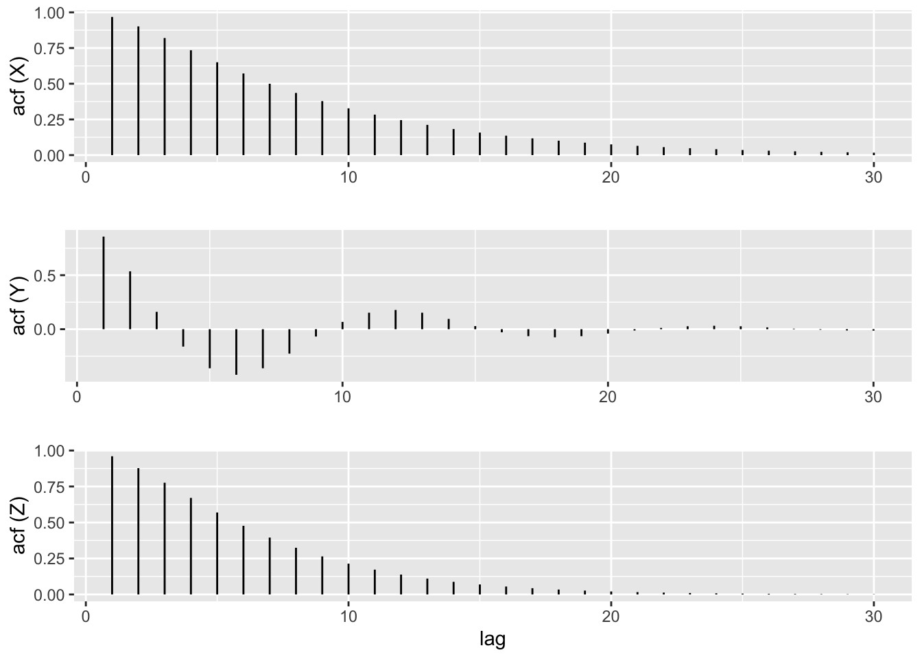

Figure 10.8: ACF plots for the AR(2) models X (top panel), Y (middle panel), Z (bottom panel), corresponding to AR polynomials with two real roots, two complex roots, and a repeated real root respectively.

10.6 Forecasts

10.6.1 Gaussian conditional distributions

We first discuss some properties of multivariate normal distributions.

Proposition 10.6. (Conditional distribution) Let \((X_1,X_2,\ldots,X_{n+1}) \sim N(\mu, \Sigma)\) be a multivariate Gaussian random vector, then given observations \(X_1=x_1, X_2 = x_2,\ldots,X_{n} = x_{n}\), the conditional distribution of \(X_{n+1}\) conditioned on these values is \[ N(\mu_{n+1} + \Sigma_{1:n,n+1}^T\Sigma_{1:n,1:n}^{-1}(x_{1:n} - \mu_{1:n}), \Sigma_{n+1,n+1} - \Sigma_{1:n,n+1}^T\Sigma_{1:n,1:n}^{-1}\Sigma_{1:n,n+1}), \] where \(\Sigma_{1:n,1:n}\) is the top left \(n \times n\) submatrix of \(\Sigma\), \(\Sigma_{n+1,n+1}\) its bottom right entry, and \(\Sigma_{n+1,1:n}\) its bottom row without the bottom right entry，i.e. \[ \Sigma = \left[\begin{matrix} \Sigma_{1:n,1:n} & \Sigma_{1:n,n+1} \\ \Sigma_{n+1,1:n} & \Sigma_{n+1,n+1} \end{matrix}\right]. \]

Proof. This is a well-known property of multivariate Gaussian distributions and can be proved by computing the conditional density using the block matrix inverse formula.

This formula is used often in many areas of statistics (and engineering). In the context of time series analysis, we typically assume stationarity, which means that the formula simplifies.

Corollary 10.7 (Conditional distribution under stationarity) Let \((X_1,X_2,\ldots)\) be a zero mean stationary Gaussian process, then given observations \(X_1=x_1, X_2 = x_2,\ldots,X_{n} = x_{n}\), the conditional distribution of \(X_{n+h}\) conditioned on these values is \[ N(\gamma_{h:n+h-1}^T\Gamma_{n}^{-1}x_{n:1}, \gamma_X(0) - \gamma_{h:n+h-1}^T\Gamma_{n}^{-1}\gamma_{h:n+h-1}), \tag{10.20}\] where \[ \gamma_{a:b} \coloneqq \left(\gamma_X(a), \gamma_X(a+1),\ldots,\gamma_X(b)\right) \tag{10.21}\] for any \(a < b\), \[ \Gamma_n \coloneqq (\gamma_X(i-j))_{i,j=1}^n, \tag{10.22}\] and \(x_{n:1} = (x_n, x_{n-1},\ldots,x_1)\).

Assuming Gaussian white noise, Equation 10.20 thus gives the distributional forecast and can be used to supply point forecasts \[ \hat x_{n+h|n} = \gamma_{h:n+h-1}^T\Gamma_{n}^{-1}x_{n:1} \tag{10.23}\] as well as 95% prediction intervals \((\hat x_{n+h|n} - 1.96v_{n+h}^{1/2}, \hat x_{n+h|n} + 1.96v_{n+h}^{1/2})\) for \(v_{n+h} = \gamma_X(0) - \gamma_{h:n+h-1}^T\Gamma_{n}^{-1}\gamma_{h:n+h-1}\).

10.6.2 Best linear predictors

The point forecast Equation 10.23 is the mean of the conditional distribution and can be thought of as a function of the random variables, i.e. \[ r(x_{1:n}) \coloneqq \E\lbrace X_{n+h}|X_1 = x_1,\ldots,X_n = x_n\rbrace. \] Conditional means are Bayes optimal predictors with respect to squared loss, i.e. we have \[ r = \textnormal{argmin}_{f \colon \R^n \to \R} \E\left\lbrace (f(X_{1:n}) - X_{n+h})^2\right\rbrace. \] This property is true for any multivariate distribution. What is special about Gaussian distributions is that the conditional mean function is linear, i.e \(r(x_{1:n}) = \phi_{n+h|n}^Tx_{n:1}\), where \[ \phi_{n+h|n} \coloneqq \Gamma_n^{-1}\gamma_{h:n+h-1}. \tag{10.24}\]

The notation \(\phi_{n+h|n}\) is purposely suggestive and will be further explained shortly. For now, we observe that \(r(X_1,X_2,\ldots,X_n)\) is also the best linear predictor (BLP) of \(X_{n+h}\) given \(X_1,X_2,\ldots,X_n\), i.e. \[ \phi_{n+h|n} = \textnormal{argmin}_{\beta \in \R^n} \E\left\lbrace (\beta^TX_{n:1} - X_{n+h})^2\right\rbrace. \tag{10.25}\]

Proposition 10.8. (BLP formula) Equation 10.24 solves Equation 10.25 even when we do not assume Gaussianity.

Proof. To see this, we simply expand out the square on the right hand side of Equation 10.25 and take a derivative with respect to \(\beta\): \[ \nabla_\beta \E\left\lbrace (\beta^TX_{n:1} - X_{n+h})^2\right\rbrace = 2\Gamma_n\beta - 2\gamma_{h:n+h-1}.~\Box \]

In general, the BLP may be different from the conditional mean, and therefore less accurate. Nonetheless, they are easy to calculate because they depend only on the second-order moments of the stochastic process. They thus provide an extremely useful forecasting framework. As we will see, forecasting in ARIMA modeling is based on the BLP principle.

Note

Generally, conditional means for multivariate Gaussians are equivalent to BLPs. This is the well-known connection between the Gaussian distribution and linear regression.

10.6.3 One-step-ahead forecasts

Notice that the \(\textnormal{AR}(p)\) formula Equation 10.6 expresses \(X_t\) as a linear function of \(X_1,X_2,\ldots,X_{t-1}\) up to additive white noise whenever \(t > p\). More precisely, if we denote \[ \tilde\phi_{t|t-1} \coloneqq (\phi_1,\phi_2,\ldots,\phi_p, 0, \ldots)^T, \] then Equation 10.6 can be written as \[ X_t = \tilde\phi_{t|t-1}^TX_{t-1:1} + W_t . \tag{10.26}\] As such, the following proposition should be unsurprising.

Proposition 10.9. (BLP for AR(p)) If \((X_1,X_2,\ldots)\) follow an \(\textnormal{AR}(p)\) model and \(t > p\), we have \(\phi_{t|t-1} = \tilde\phi_{t|t-1}\).

Proof. Multiply Equation 10.26 on the right by \((X_{t-1},X_{t-2},\ldots,X_1)\) and take expectations. We get \[ \gamma_{1:t-1}^T = \tilde\phi_{t|t-1}^T\Gamma_{t-1} \] Now multiplying both sides on the right by \(\Gamma_{t-1}^{-1}\) and take transposes. The resulting expression is equal to Equation 10.24, when selecting \(h=1, n=t-1\), which completes the proof. \(\Box\)

As such, while the one-step-ahead BLP could a priori be a function of all past observations, in the case of an \(\textnormal{AR}(p)\) model, it only relies on the most recent \(p\) observations and can be written as the vector of model parameters (padded with zeros.)

10.6.4 Recursive forecasts

We have already seen how to forecast \(h\) steps ahead by directly minimizing the squared loss in Equation 10.25. This approach is sometimes called direct multi-step forecasting, to contrast it with another approach called recursive multi-step forecasting. In recursive forecasting, we recursively forecast one step ahead at a time, using the previously forecasted values as inputs for each subsequent forecast.

For instance, given observations \(x_1,x_2,\ldots,x_n\) and \(n \geq p\), we forecast \[ \begin{split} \hat x_{n+1|n} & \coloneqq \phi^T(x_n, x_{n-1},\ldots,x_{n-p+1}), \\ \hat x_{n+2|n} & \coloneqq \phi^T(\hat{x}_{n+1|n}, x_n, x_{n-1},\ldots,x_{n-p+2}), \\ \hat x_{n+3|n} & \coloneqq \phi^T(\hat{x}_{n+2|n}, \hat{x}_{n+1|n}, x_n,\ldots,x_{n-p+3}), \end{split} \tag{10.27}\] and so on.

More generally, recursive forecasting turns a method for generating one-step-ahead forecasts into a method for generating forecasts for any time horizon. It is thus a particularly useful approach for time series models based on machine learning, with comparisons between recursive and direct approaches being a topic of discussion and research. For \(\textnormal{AR}(p)\) models, however, both approaches provide the exact same forecasts.

Proposition 10.10. For an \(\textnormal{AR}(p)\) model, both recursive and direct multi-step forecasts are the same.

Proof. In order to distinguish them from direct forecasts, we temporarily refer to the recursive forecasts defined in Equation 10.13 using the notation \(\tilde x_{n+h|n}\) for \(h=1,2,\ldots\).

The key observation is that random variables⁶ form an inner product space with covariance as the inner product. The BLP of \(X_{n+h}\) given \(X_1,X_2,\ldots,X_n\) can be interpreted as the orthogonal projection of \(X_{n+h}\) onto the linear span of these random variables. Let us denote this projection operator as \(Q_n\). We now induct on \(h\), with the base case \(h=0\) trivial. For the induction step, we compute:

\[ \begin{split} \hat X_{n+h+1|n} & \coloneqq Q_n[X_{n+h+1}] \\ & = Q_n[\phi_1 X_{n+h} + \cdots + \phi_p X_{n+h-p+1} + W_{n+h+1}] \\ & = \phi_1 Q_n[X_{n+h}] + \cdots \phi_p Q_n[X_{n+h-p+1}] \\ & = \phi_1 \tilde X_{n+h|n} + \phi_p \tilde X_{n+h-p+1|n} \\ & \eqqcolon \tilde X_{n+h+1|n}, \end{split} \] where the second last equality follows from the induction hypothesis.

Note that this is a statement of equality between two random variables. Conditioning on the values \(X_1=x_1,X_2=x_2,\ldots,X_n=x_n\) turns the upper case \(X\)’s into lower cases \(x\)’s. \(\Box\)

Note

We have stated almost all results in this section under the assumption that \((X_t)\) has mean \(\mu = 0\). More generally, when the model has nonzero mean, we first apply the results for the translation \(Y_t \coloneqq X_t - \mu\), and then add \(\mu\) to get the forecast for \(X_t\).

10.7 Estimation

In order to apply \(\textnormal{AR}(p)\) models to real data, we have to first estimate the \(p+2\) model parameters: \(\mu, \phi_1,\phi_2,\ldots,\phi_p,\sigma^2\). Estimating these parameters is also called fitting the model.

We have seen that exponential smoothing models were fit by minimizing the sum of squared errors (see Equation 8.2) for one-step-ahead forecasts, i.e. the model residuals. This is also a valid approach for estimating \(\textnormal{AR}(p)\) models. In addition to this, we introduce two other methods which are commonplace in statistics: the method of moments and the method of maximum likelihood.

10.7.1 Method of moments

The basic idea of the method of moments in parametric estimation is to compute the sample moments (expectation, variance, etc.) of the data and then to find the parameters of the model whose population moments match the sample moments. It is easy to implement this idea for \(\textnormal{AR}(p)\) models.

Recall that when we introduced Equation 10.14 and Equation 10.15, we used them to express the ACVF of an \(\textnormal{AR}(p)\) model in terms of its model parameters. Conversely, they also express the model parameters in terms of the ACVF. They are called the Yule-Walker equations and we reproduce them here in a more convenient form:⁷ \[ \phi = \Gamma_p^{-1}\gamma_{1:p}, \quad\quad \sigma^2 = \gamma(0) - \gamma_{1:p}^T\Gamma_p^{-1}\gamma_{1:p}. \] Note that \(\gamma_{1:p}\) and \(\Gamma_p\) are defined in Equation 10.21 and Equation 10.22 respectively.

The method of moment estimators or Yule-Walker estimators for the parameters are defined via \[ \hat \phi \coloneqq \hat\Gamma_p^{-1}\hat\gamma_{1:p}, \quad\quad \hat\sigma^2 \coloneqq \hat\gamma(0) - \hat\gamma_{1:p}^T\hat\Gamma_p^{-1}\hat\gamma_{1:p}, \] where \(\hat\gamma_{1:p}\) and \(\hat\Gamma_p\) are defined in terms of the sample ACVF values. The mean \(\mu\) is estimated using the sample mean \(\bar x_{1:n}\).

Note that the method of moments is well-defined even when we do not assume Gaussian white noise. Although we didn’t give it a name at the time, this was also the method we introduced for estimating the model parameters for \(\textnormal{AR}(1)\).

Note

We do not need to consider higher order moments because the \(\textnormal{AR}(p)\) model is fully determined by its mean and ACVF.

10.7.2 Method of maximum likelihood

The maximum likelihood estimator (MLE) is the parameter value that maximizes the likelihood function given the observed data. When using this method for stationary time series models, we usually assume Gaussian white noise, which means that the model (\(\textnormal{AR}(1)\) or otherwise) is a Gaussian process.

Full MLE. Using Equation 10.6 and the causality assumption, we may write conditional densities as \[ f_\beta(x_t|x_1,\ldots,x_{t-1}) = (2\pi\sigma^2)^{-1/2}\exp\left(-\frac{(x_t - \phi_{1:p}^T(x_{t-1:t-p} -\mu) - \mu)^2}{2\sigma^2}\right) \] whenever \(t > p\). Here, we use \(\beta = (\mu, \phi_{1:p},\sigma^2)\) to denote the entire vector model parameters. For \(1 \leq t\leq p\), we have the more complicated expression \[ f_\beta(x_t|x_1,\ldots,x_{t-1}) = (2\pi\nu_t^2)^{-1/2}\exp\left(-\frac{(x_t - \phi_{1:t-1}^T(x_{t-1:1} -\mu) - \mu)^2}{2\nu_t^2}\right), \] where \(\nu_t^2 = \gamma(0) - \gamma_{1:t-1}^T\Gamma_{t-1}^{-1}\gamma_{1:t-1}\) (see Corollary 10.7) and the ACVF values \(\gamma(k)\) are treated as functions in \(\beta\) obtained via Equation 10.14 and Equation 10.15.

Taking logarithms, we therefore get the following expression for the negative log likelihood: \[ \begin{split} l(\beta) & = - \log f_\beta(x_1,x_2,\ldots,x_n) \\ & = -\log \prod_{t=1}^n f_\beta(x_t|x_1,\ldots,x_{t-1}) \\ & = \frac{n}{2}\log(2\pi\sigma^2) + \frac{1}{2}\sum_{t=1}^p \log (\nu_t^2/\sigma^2) + \frac{S(\mu, \phi_{1:p})}{2\sigma^2} \end{split} \tag{10.28}\] where \[ \begin{split} S(\mu, \phi_{1:p}) & = \sum_{t=1}^p (x_t - \mu - \phi_{1:t-1}^T(x_{t-1:1} -\mu))^2\cdot\frac{\sigma^2}{\nu_t^2} \\ & \quad\quad + \sum_{t=p+1}^n (x_t - \mu - \phi_{1:p}^T(x_{t-1:t-p} -\mu))^2. \end{split} \tag{10.29}\]

Note that \(\sigma^2/\nu_t^2\) is purely a function of \(\phi_{1:p}\) and does not depend on \(\sigma^2\).

The MLE is defined as the minimizer of Equation 10.28. But because of the presence of \(\nu_1,\nu_2,\ldots\), Equation 10.28 is a complicated function of \(\beta\), and can only be minimized numerically.

Conditional MLE. The likelihood can be greatly simplified by conditioning on the first \(p\) values: \(X_1 = x_1, X_2 = x_2, \ldots,X_p = x_p\). The conditional negative log likelihood is then \[ \begin{split} l_c(\beta) & \coloneqq - \log f_\beta(x_{p+1},x_{p+2},\ldots,x_n|x_1,x_2,\ldots,x_p) \\ & = -\log \prod_{t=p+1}^n f_\beta(x_t|x_1,\ldots,x_{t-1}) \\ & = \frac{n-p}{2}\log(2\pi\sigma^2) + \frac{S_c(\mu, \phi_{1:p})}{2\sigma^2} \end{split} \tag{10.30}\] where \[ \begin{split} S_c(\mu, \phi_{1:p}) & = \sum_{t=p+1}^n (x_t - \mu - \phi_{1:p}^T(x_{t-1:t-p} -\mu))^2. \end{split} \tag{10.31}\]

By differentiating Equation 10.30 with respect to \(\sigma^2\), we see that the MLE for \(\sigma^2\) is \[ \hat\sigma^2 = \frac{S_c(\hat\mu,\hat\phi_{1:p})}{n-p}, \] where \(\hat\mu\) and \(\hat\phi_{1:p}\) are the MLEs for \(\mu\) and \(\phi_{1:p}\) respectively.

Next, differentiating \(S_c(\mu, \phi_{1:p})\) with respect to \(\mu\) and \(\phi\), we get \[ \hat\phi = \tilde\Gamma_p^{-1}\tilde\gamma_{1:p} \] and \[ \hat\mu = \frac{\bar x_{p+1:n} - \hat\phi_1 \bar x_{p:n-1} - \cdots - \hat\phi_p \bar x_{1:n-p}}{1 - \hat\phi_1 - \cdots - \hat\phi_p}. \] Here \(\bar x_{a:b} = \frac{1}{b-a+1}\sum_{i=a}^b x_i\) for any \(a < b\). Furthermore, the entries of \(\tilde\Gamma_p\) and \(\tilde\gamma_{1:p}\) are of the form \[ (\tilde\Gamma_p)_{ij} = \frac{1}{n-p}(x_{p-i+1:n-i} - \bar x_{p-i+1:n-i})^T(x_{p-j+1:n-j} - \bar x_{p-j+1:n-j}), \] \[ \tilde\gamma(i) = \frac{1}{n-p}(x_{p-i+1:n-i} - \bar x_{p-i+1:n-i})^T(x_{p+1:n} - \bar x_{p+1:n}). \]

10.7.3 Least squares

Conditional least squares. We have just seen that the MLE is the minimizer of \(S_c(\mu,\phi)\), defined in Equation 10.31. This objective function is called the conditional sum of squares and comprises the sum of the squared one-step-ahead errors. While the likelihood function may change under other choices of the white noise distribution, just like in linear regression, \(S_c(\mu,\phi)\) remains a reasonable objective function for fitting the model parameters.

Unconditional least squares. Another objective function of interest is the unconditional sum of squares \(S(\mu,\phi)\), defined in Equation 10.29. This forms part of the full likelihood in Equation 10.28, but because the likelihood includes an additional logarithmic term depending on \(\nu_t^2/\sigma^2\), the two objectives have different minimizers.

10.7.4 Asymptotics

We have introduced four different estimators:

• Method of moments
• Full maximum likelihood
• Conditional maximum likelihood / conditional sum of squares minmizer
• Unconditional sum of squares minimizer

Given these possibilities, it is natural to ask which estimator is the most efficient, i.e. which converges to the true parameters at the fastest rate. It turns out that for \(\textnormal{AR}(p)\) models, all four are asymptotically equivalent and optimal.

Theorem 10.11. (Large sample distribution of estimators) Suppose the white noise has finite 4th moments, i.e. \(\E\lbrace W_t^2\rbrace < \infty\). Then for each of the four estimators listed above, \(\hat\sigma^2\) is consistent and \[ \sqrt n (\hat\phi_{1:p} - \phi_{1:p}) \to_d N(0,\sigma^2\Gamma_p^{-1}). \]

Proof. It is not hard to see that the three estimators based on likelihood are equivalent, since the objective functions by which they are defined differ by an \(O(1/n)\) additive factor as \(n \to \infty\). We can also compare the method of moments estimator with the conditional max likelihood estimator using a similar reasoning: For instance, we see that the entries of \(\hat \Gamma_p\) and \(\tilde\Gamma_p\) also differ by an \(O(1/n)\) additive factor. Refer to Section B.3. in Shumway and Stoffer (2000) for the remaining details of the proof.

Note that the Cramer-Rao lower bound implies that \(\sigma^2\Gamma_p^{-1}\) is the optimal asymptotic covariance.

Using Theorem 10.11, we are able to provide confidence intervals and perform hypothesis testing for model parameters. Of course, confidence intervals rely on assuming that all the modeling assumptions hold and that we know the correct order \(p\) for the model. This is rarely the case for real data analysis. At the very least, one ought to be able to estimate the model order without knowing it before hand. This is called model selection and will be discussed in the next chapter.

10.8 Sample trajectories

One can draw a sample trajectory from an autoregressive model (and more generally from an ARIMA model) using the function arima.sim() in base R. Here, we show sample trajectories from the \(\textnormal{AR}(2)\) models \((X_t)\), \((Y_t)\), and \((Z_t)\) whose ACF we computed in Figure 10.8. We also plot forecasts over 20 time steps.

set.seed(5209)
n <- 80
h <- 20
ar2_data <-
    tibble(t = 1:n,
           wn = rnorm(n),
1           X = arima.sim(model = list(ar = c(1.5, -0.55)),
                         n = n, innov = wn),
           Y = arima.sim(model = list(ar = c(1.5, -0.75)), 
                         n = n, innov = wn),
           Z = arima.sim(model = list(ar = c(1.5, -0.5625)), 
                         n = n, innov = wn)
    ) |>
    as_tsibble(index = t)
plt1 <- ar2_data |>
2    model(X = ARIMA(X ~ pdq(2, 0, 0))) |>
    forecast(h = h) |>
    autoplot(ar2_data) + ylab("X")
plt2 <- ar2_data |>
    model(Y = ARIMA(Y ~ pdq(2, 0, 0))) |>
    forecast(h = h) |>
    autoplot(ar2_data) + ylab("Y")
plt3 <- ar2_data |>
    model(Z = ARIMA(Z ~ pdq(2, 0, 0))) |>
    forecast(h = h) |>
    autoplot(ar2_data) + ylab("Z")
grid.arrange(plt1, plt2, plt3, nrow = 3)

1

arima.sim() creates a sample trajectory from an ARIMA model. We first specify the model parameters as a list with only one item, which we name ar, set the desired trajectory length to be \(n = 80\), and request that it be generated using the white noise sequence wn. We use the same white noise sequence for all three models in order to have a better comparison among them.

2

To forecast using the fable package, we first fit a model to the data using the ARIMA() function. Since we already know the model parameters, we don’t have to do this, but we proceed in order to make use of the resulting mable interface.

Figure 10.9: Sample trajectories and forecasts for AR(2) models with phi_1 = 1.5 but different values of phi_2. These are (from top to bottom) -0.55, -0.75 and -0.5625. The noise variance is set to be 1.

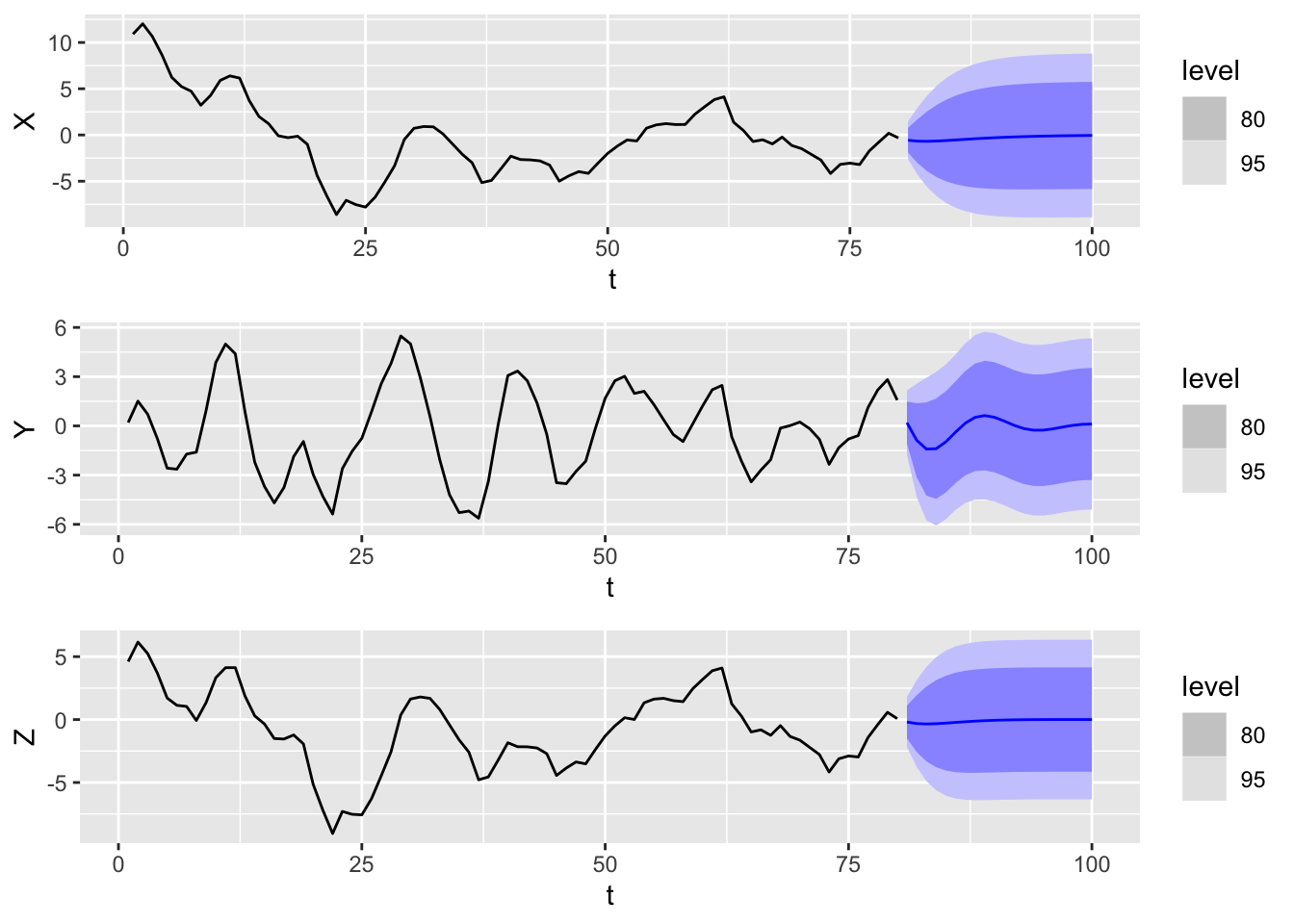
From the plots, we see that \((Y_t)\) has cycles whereas \((X_t)\) and \((Z_t)\) do not. This is unsurprising as the AR polynomial defining \((Y_t)\) has complex roots whereas those defining \((X_t)\) and \((Z_t)\) do not.

When arima.sim() is called with a choice of parameters that do not produce a causal, stationary model, it throws an error.

#> This is not causal
arima.sim(model = list(ar = 1.1), n = 50)

Error in arima.sim(model = list(ar = 1.1), n = 50): 'ar' part of model is not stationary

Nonetheless, we can try to compute this manually using the base R function accumulate(). Doing so gives the following plot.

set.seed(5209)
n <- 50
wn <- rnorm(n - 1)
tibble(t = 1:n,
       X = accumulate(wn, ~ 1.1 * .x + .y, .init = 0)
    ) |>
    as_tsibble(index = t) |>
    autoplot(X)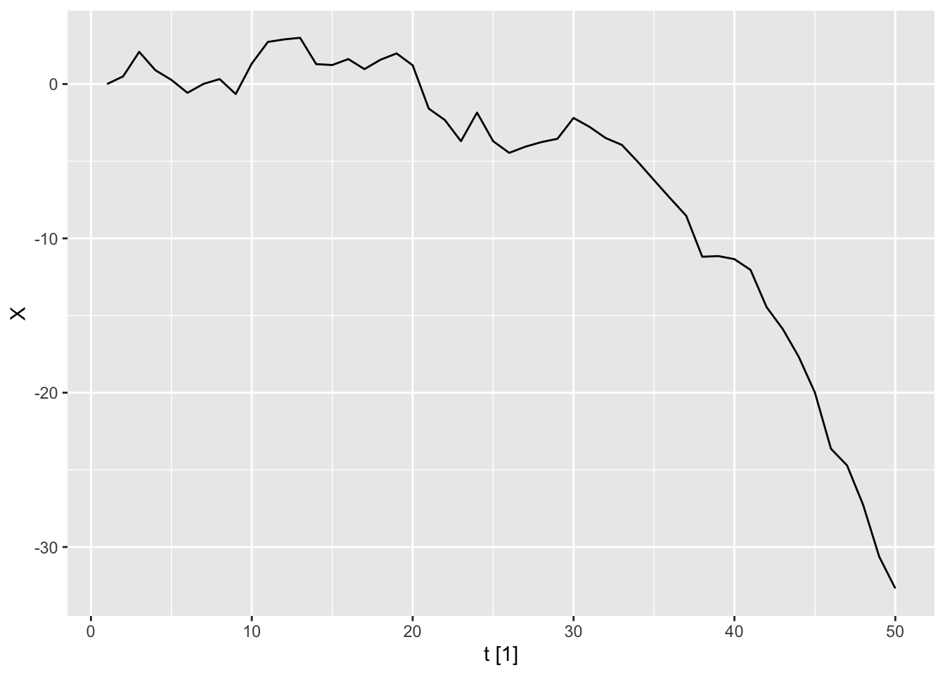

Figure 10.10: Sample trajectory for an explosive AR(1) model.

We see that the time series diverges exponentially. Note that our method of sampling trajectories (also used by arima.sim()) implicitly assumes that the future white noise values are independent of the past values of the process. Hence, it generates the explosive solution for non-causal AR(1) model rather than the stationary one.

10.9 Nonlinear autoregressive models

In this chapter, we have discussed \(\textnormal{AR}(p)\) models at length. Although we sometimes call these autoregressive models, they are more accurately described as linear autoregressive models, because they stipulate that each value \(X_t\) depends on the past values linearly. Just as in supervised learning, there can be nonlinear dependence between the values of a time series, which cannot be captured by a linear model.

When encountering such patterns, it may be fruitful to apply autoregressive machine learning models, which are machine learning models that take lagged covariates as predictors. These are usually optimized by minimizing the sum of squared residuals. fable conveniently comes equipped with neural network autoregressive models (see Chapter 12.4 in Hyndman and Athanasopoulos (2018)), but any regression model can be turned into an autoregressive model.

Hyndman, Rob J, and George Athanasopoulos. 2018. Forecasting: Principles and Practice. OTexts.

Shumway, Robert H, and David S Stoffer. 2000. Time Series Analysis and Its Applications. Vol. 3. Springer.

Yule, G. Udny. 1927. “On a Method of Investigating Periodicities in Disturbed Series, with Special Reference to Wolfer’s Sunspot Numbers.” Philosophical Transactions of the Royal Society of London. Series A, Containing Papers of a Mathematical or Physical Character 226: 267–98. https://www.jstor.org/stable/91170.

---

1. Exactly what this noise comprises of seems to be a topic of current research.

2. We omit the constant term in the equation due to our remarks in the previous section.

3. Because of this lack of independence, we cannot use the equations in Section 10.3.3 to forecast or simulate sample trajectories.

4. If we relax the condition to \(\phi(z) \neq 0\) for all \(|z| = 1\), unique stationary solutions still exist, but they may be noncausal. We do not discuss this case.

5. We may always factorize \(\phi\) this way, according to the fundamental theorem of algebra.

6. More accurately, the space of zero mean random variables that have finite variance and that are measurable with respect to the sigma algebra generated by the time series.

7. The second equation is derived by plugging in the first equation (in matrix form) into Equation 10.15.