A moving average model of order \(q\), abbreviated \(\textnormal{MA}(q)\), is a stationary stochastic process \((X_t)\) defined via \[
X_t = \mu + W_t + \theta_1 W_{t-1} + \theta_2 W_{t-2} + \cdots + \theta_q W_{t-q},
\tag{11.1}\] where \((W_t) \sim WN(0,\sigma^2)\), and \(\theta_1,\theta_2,\ldots,\theta_q\) are constant coefficients.
The sequence \((X_t)\) can be thought of as a moving average of the current and \(q\) most recent white noise values, hence the name. On the other hand, the weights \(\theta_j\) can be negative, as opposed to what happens when we use moving averages to smooth a time series.
\(\textnormal{MA}(q)\) models possess a nice symmetry with \(\textnormal{AR}(p)\) models. If we define the moving average polynomial to be \[
\theta(z) = 1 + \theta_1 z + \theta_2 z^2 + \cdots + \theta_q z^q,
\] then we may rewrite Equation 11.1 in operator form as \[
X_t - \mu = \theta(B)W_t,
\] where \(B\) is the backshift operator as before. We call \(\theta(B)\) the moving average operator of the model.
11.1.2 Motivation: Lagged effects
When modeling the influence of one time series on another, it is important to account for lagged effects. For instance, if a company runs a successful marketing campaign in March, it may experience higher sales numbers starting in April and persisting for the rest of the year. Similarly, the population size of a predator species depends on the population size of its prey in a lagged manner (see for instance the cross-correlation plot in Figure 6.10.)
One can interpret Equation 11.1 as asserting a driving relationship with lagged effects between \((W_t)\) and an observed time series \((X_t)\). Of course, this assumes that the driver is white noise, which is not always reasonable. Nonetheless, \(\textnormal{MA}(q)\) models may provide a building block for more complicated models, as we will soon see.
11.1.3 Similarities with AR(p) models
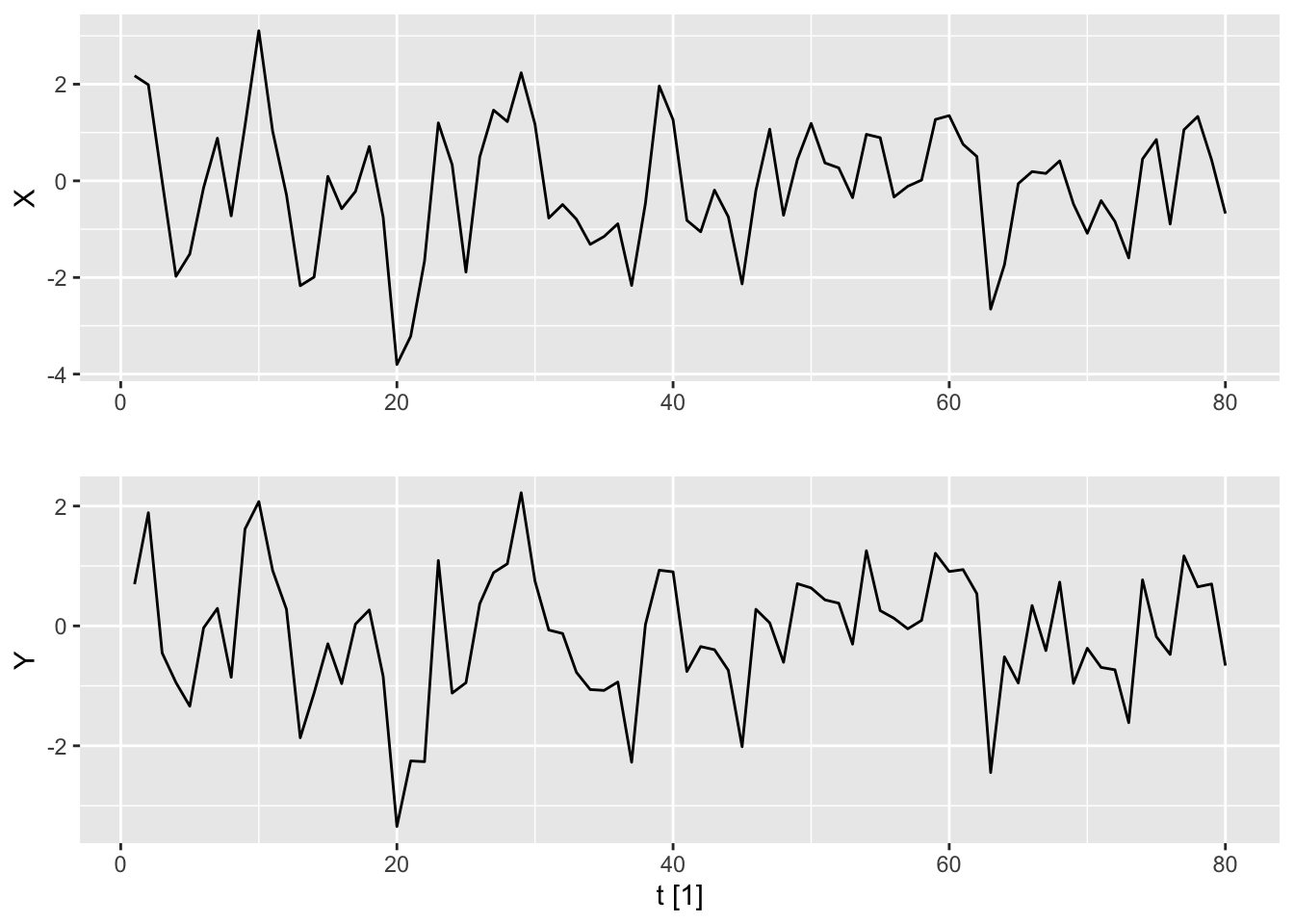
It can be hard to distinguish between sample trajectories of \(\textnormal{AR}(p)\) and \(\textnormal{MA}(q)\) models using the naked eye. We plot here samples from the models \[
X_t = W_t + 0.9W_{t-1}
\]\[
Y_t = 0.5Y_{t-1} + W_t,
\] generated using the same white noise process. Note that the first model is an \(\textnormal{MA}(1)\) model, while the second is an \(\textnormal{AR}(1)\) model. Their parameters are selected so that they have similar ACVF values (see Section 11.1.5.)
Figure 11.1: Sample trajectories and forecasts for an MA(1) model with theta = 0.9 (top) and an AR(1) model with phi = 0.5 (bottom).
Second, if we allow for infinite order, then both classes of models are equivalent. We have already seen that causal \(\textnormal{AR}(p)\) models are equivalent to \(\textnormal{MA}(\infty)\) models. Likewise, under some conditions, we may show that an \(\textnormal{MA}(q)\) model is also an \(\textnormal{AR}(\infty)\) model.
Invertibility. We say that a stochastic process \((X_t)\) is invertible if it satisfies the equation \[
\sum_{j=0}^\infty \pi_j (X_{t-j} - \mu) = W_t
\tag{11.2}\] where \(\sum_{j=0}^\infty |\pi_j| < \infty\).
Proposition 11.1. Let \((X_t)\) be an \(\textnormal{MA}(q)\) model with MA polynomial \(\theta(z)\). Suppose \(\theta(z) \neq 0\) for all \(|z| \leq 1\). Then \((X_t)\) is invertible, with coefficients satisfying \[
\theta(z) \cdot \left( \sum_{j=0}^\infty \pi_j z^j\right) = 1.
\tag{11.3}\]
The proof of this proposition is similar to that of Theorem 10.4 and is left to the reader. The important point to note is that Equation 11.3 yields a recursive formula for \(\pi_j\), \(j=0,1,2,\ldots\).
11.1.4 Differences with AR(p) models
In comparison with \(\textnormal{AR}(p)\) models, we do not have to worry about whether Equation 11.1 gives a well-defined model—the model is explicitly defined by the equation. On the other hand, forecasting and estimation become more difficult. Simply viewing an \(\textnormal{MA}(q)\) model as an \(\textnormal{AR}(\infty)\) model is not too helpful, because the order of the AR model matters for forecasting and estimation.
Forecasting:For \(\textnormal{AR}(p)\), only the past \(p\) observations are relevant.
Estimation: \(\textnormal{AR}(p)\) requires estimating the \(p\)-dimensional matrix \(\Gamma_p\).
Neither of these are feasible when \(p = \infty\) and we have to work with \(\textnormal{MA}(q)\) directly. Here, we note that although Equation 11.1 seems similar to a regression equation, we do not actually observe the white noise values \(W_t, W_{t-1},\ldots\) when modeling real data and cannot use them for prediction or estimation.
11.1.5 Moments
The mean of Equation 11.1 is \(\mu\). Meanwhile, the ACVF is given by Equation 9.4: \[
\gamma_X(h) = \begin{cases}
\sigma^2\sum_{j=h}^q \theta_j\theta_{j-h} & 0 \leq h \leq q \\
0 & h > q.
\end{cases}
\]
Dividing by the formula for \(\gamma_X(0)\) gives \[
\rho_X(h) = \begin{cases}
\frac{\sum_{j=h}^q \theta_j\theta_{j-h}}{\sum_{j=0}^q \theta_j^2} & 0 \leq h \leq q \\
0 & h > q.
\end{cases}
\]
In contrast with the gradual decay of ACF values for \(\textnormal{AR}(p)\) models, we see that the ACF for \(\textnormal{MA}(q)\) experience a sharp cutoff after \(q\) lags.
Given these moments, we can forecast using the best linear predictor formula Equation 10.20. On the other hand, this formula requires estimating and inverting the \(n\)-dimensional matrix \(\Gamma_n\), neither of which is desirable. We were able to get around this for \(\textnormal{AR}(p)\), in which case the BLP formula conveniently simplifies to only depend on the \(p\) most recent observations. Unfortunately, this is not the case for \(\textnormal{MA}(q)\) models, as we will see in the next section.
11.2 Partial autocorrelation function
In order to further discuss issues with forecasting, we introduce a counterpart to the ACF: The partial autocorrelation function, or PACF for short. It is based on partial correlation, which is a concept from regression analysis that is important in its own right.
11.2.1 Partial correlation
Let \(\bZ = (Z_1,\ldots,Z_m)\) be a random vector, and let \(X\) and \(Y\) be two additional random variables. Let \(\hat X\) and \(\hat Y\) be the best linear predictors for \(X\) and \(Y\) respectively given \(\bZ\).1 Then the partial correlation between \(X\) and \(Y\) given \(\bZ\) is \[
\rho_{X,Y|\bZ} \coloneqq \Corr\left\lbrace X-\hat X, Y - \hat Y\right\rbrace.
\]
In regression analysis, the residuals \(X - \hat X\) and \(Y - \hat Y\) represent the remaining variation in \(X\) and \(Y\) respectively after controlling for the effect of \(\bZ\). Any correlation between these residuals is often more interesting than that between the original \(X\) and \(Y\). For instance, although a strong correlation between smoking and lung cancer has long been observed, prominent statisticians such as Ronald Fisher once tried to argue that there were other variables, such as genetic factors, that led to both a higher incidence of smoking and a higher incidence of lung cancer.2 His hypothesis could be refuted if we were able to show a positive partial correlation between smoking and lung cancer after controlling for these genetic factors.
Caution
Do not confuse partial correlation with conditional correlation, which measures the correlation between the residuals \(X - \hat X\) and \(Y - \hat Y\) where \(\hat X\) and \(\hat Y\) are now the conditional expectations of \(X\) and \(Y\) given \(\bZ\) (rather than the BLP). Partial correlation and conditional correlation are equivalent when \(\bZ\), \(X\) and \(Y\) are jointly multivariate Gaussian.
Regression coefficient. If we regress \(Y\) jointly on \(\bZ\) and \(X\), then the regression coefficient of \(X\) is \[
\beta_X = \rho_{X,Y|\bZ}\cdot \sqrt{\frac{\Var\lbrace Y - \hat Y\rbrace}{\Var \lbrace X - \hat X\rbrace}}.
\tag{11.4}\]
Analysis of variance. Let \(\hat Y\) be the BLP of \(Y\) using \(\bZ\) and let \(\tilde Y\) be the BLP of \(Y\) using both \(\bZ\) and \(X\). Then \[
\rho_{X,Y|\bZ}^2 = 1 - \frac{\Var\lbrace Y - \tilde Y\rbrace}{\Var\lbrace Y - \hat Y\rbrace}.
\tag{11.5}\]
Proof.Equation 11.4 can be proved by checking that \(\hat Y + \beta_X(X - \hat X)\) is the BLP for \(Y\) given \(\bZ\) and \(X\) using the zero gradient condition. Equation 11.5 is obtained by rearranging the definition of \(\rho_{X,Y| \bZ}\).
Under both interpretations, we see that a nonzero partial correlation implies that knowing \(X\) improves our prediction accuracy for \(Y\) even if we already know \(\bZ\).
11.2.2 Defining PACF
The lag \(h\) partial autocorrelation of a stationary process \((X_t)\) is defined as the partial correlation between \(X_0\) and \(X_h\) given \(X_1,X_2,\ldots,X_{h-1}\).3 In other words, it is \[
\alpha_X(h) \coloneqq \rho_{X_0,X_{h}|X_{1:h-1}}.
\]
\(\alpha_X\) is called the partial autocorrelation function, or PACF for short. Note that it is not defined for \(h = 0\) and that \(\alpha_X(1) = \rho_X(1)\) (since nothing is conditioned upon at lag 1.)
BLP coefficient.\(\alpha_X(h)\) is the \(h\)-th coordinate of \(\phi_{h+1|h}\), the regression vector of \(X_{h+1}\) on \(X_1,X_2,\ldots,X_h\).
Residual variance. Let \(\nu_{h+1}\) denote the residual variance of the BLP, i.e. \(\Var\lbrace X_{h+1} - \phi_{h+1|h}^T X_{h:1}\rbrace\). Then we have \[
\nu_{h+1} = (1-\alpha_X(h)^2)\nu_{h}.
\]
11.2.3 Calculating the PACF
The fact that each PACF value is equivalent to a BLP coefficient allows us to calculate it by repeatedly solving BLP equations. This procedure is made efficient using the Durbin-Levinson Algorithm. Indeed, the algorithm recursively calculates the BLP coefficient vectors \(\phi_{1|0}, \phi_{2|1}, \phi_{3|2},\ldots\) using the following proposition.
Proposition 11.2. Denote \(\phi_{t+1|t} = (\phi_{t1},\phi_{t2},\ldots,\phi_{tt})\). Then \(\phi_{00} = 0\) and for \(t = 1, 2, \ldots\), we have \[
\phi_{tt} = \frac{\rho_X(t) - \sum_{k=1}^{t-1}\phi_{t-1,k}\rho_X(t-k)}{1 - \sum_{k=1}^{t-1}\phi_{t-1,k}\rho_X(k)}
\]\[
\phi_{tk} = \phi_{t-1,k} - \phi_{tt}\phi_{t-1,t-k}, \quad k = 1,2, \ldots, t-1.
\]
Proof. These equations can be proved using the block matrix inverse formula and the observation that \[
\Gamma_t = \left[\begin{matrix}
\Gamma_{t-1} & \gamma_{t-1:1} \\
\gamma_{t-1:1}^T & \gamma_X(0)
\end{matrix}\right]
.
\]
11.2.4 AR(p) and MA(q)
The Durbin-Levinson Algorithm can be used to compute the PACF for both \(\textnormal{AR}(p)\) and \(\textnormal{MA}(q)\) models. Even without the algorithm though, we easily see that the PACF for an \(\textnormal{AR}(p)\) model is zero for all \(h > p\).4
On the other hand, for an \(\textnormal{MA}(1)\) model, we get \[
\alpha_X(h) = - \frac{(-\theta)^h(1-\theta^2)}{1-\theta^{2(h+1)}}.
\] More generally, the PACF for an \(\textnormal{MA}(q)\) undergoes exponential decay, but is nonzero for infinitely many values of \(h\). This has disappointing consequences for forecasting \(\textnormal{MA}(q)\) models: It tells us that if we would like to have a forecast that is as accurate as possible, then we will need to use all past observations of the time series that are available to us.
Caution
The intermediate coefficients \(\phi_1,\phi_2,\ldots,\phi_{p-1}\) of an \(\textnormal{AR}(p)\) model are not the PACF values for any lag \(h\). This is because the regression of \(X_n\) on \(X_{n-1}, X_{n-1},\ldots,X_{n-k}\) for any \(k < p\) is affected by omitted variable bias.
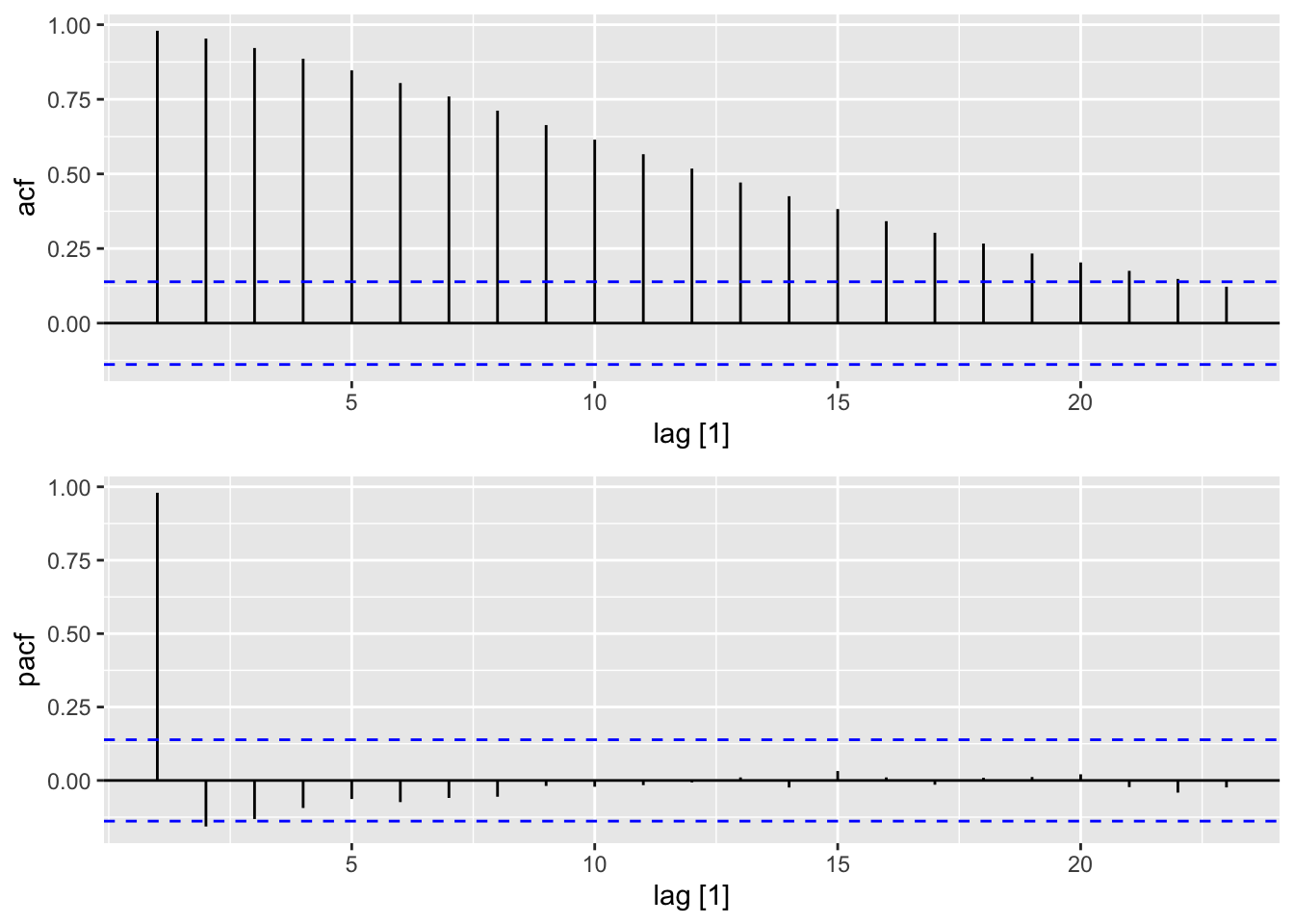
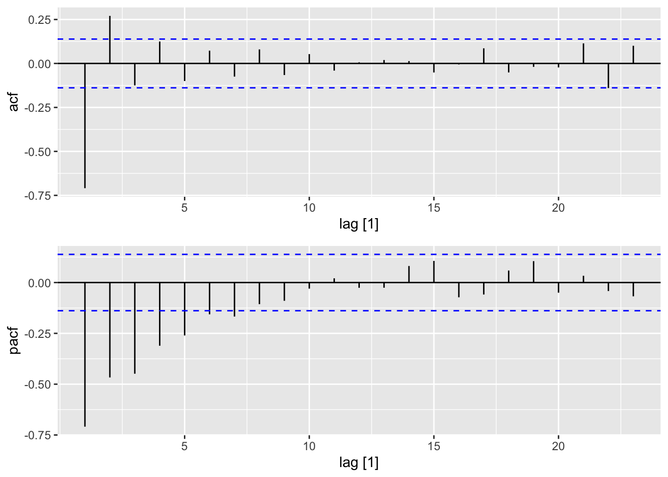
The sharp cutoffs of the ACF for \(\textnormal{MA}(q)\) models and of the PACF for \(\textnormal{AR}(p)\) models means that we can use these plots to diagnose the type and order of a model. Here, we demonstrate this for \[
\textnormal{AR}(2):\quad\quad (I - 0.9B)^2 X_t = W_t,
\]\[
\textnormal{MA}(2):\quad\quad Y_t = (I - 0.9B)^2W_t.
\]
Figure 11.3: ACF (top) and PACF (bottom) plots for an MA(2) model.
11.3 Introducing ARMA(p,q) models
11.3.1 Definitions
One may combine the definitions of \(\textnormal{AR}(p)\) and \(\textnormal{MA}(q)\) together to get an even more flexible class of models:
An autoregressive moving average model of order \(p\) and \(q\), abbreviated \(\textnormal{ARMA}(p,q)\), is a stationary stochastic process \((X_t)\) that solves the equation \[
X_t = \alpha + \phi_1 X_{t-1} + \ldots + \phi_p X_{t-p} + W_t + \theta_1 W_{t-1} + \cdots + \theta_q W_{t-q},
\tag{11.6}\] where \((W_t) \sim WN(0,\sigma^2)\) and \(\phi_1,\ldots,\phi_p,\theta_1,\ldots,\theta_q\) are constant coefficients.
In analogy with \(\textnormal{AR}(p)\) models, we can interpret Equation 11.6 as saying that \((X_t)\) is governed by an underlying dynamical system that is perturbed by noise, but in this case, the noise is described by an \(\textnormal{MA}(q)\) process rather than being white noise.
The autoregressive and moving average polynomials of the model are defined respectively as \[
\phi(z) = 1 - \phi_1 z - \phi_2 z^2 - \cdots - \phi_p z^p
\]\[
\theta(z) = 1 + \theta_1 z + \theta_2 z^2 + \cdots + \theta_q z^q,
\] and we may write Equation 11.6 in operator form as \[
\phi(B)(X_t - \mu) = \theta(B)W_t,
\tag{11.7}\] where \(\mu = \alpha/(1-\phi_1 - \cdots - \phi_p)\).
11.3.2 Parameter redundancy
Equation 11.7 demonstrates a potential issue with how \(\textnormal{ARMA}(p,q)\) are specified: If a time series \((X_t)\) satisfies the equation, then it is also a solution to \[
\eta(B)\phi(B) X_t = \eta(B)\theta(B)W_t
\] for any polynomial \(\eta\)(z). As such, we assume when writing Equation 11.6 that the autoregressive and moving average polynomials are written in their simplest possible form, i.e. that they do not share any common roots.
11.3.3 Existence, causality and invertibility
Just as with \(\textnormal{AR}(p)\) models, the equation Equation 11.6 does not a priori define a model, and we need to show that solutions exist. Furthermore, we have seen that causality and invertibility are useful properties to assume for \(\textnormal{AR}(p)\) and \(\textnormal{MA}(q)\) models respectively. These definitions are also useful for \(\textnormal{ARMA}(p,q)\) models.
Proposition 11.3. Suppose \(\phi(z) \neq 0\) for all \(|z| \leq 1\), then Equation 11.6 admits a unique stationary solution. This solution is causal and has the form \[
X_t = \mu + \sum_{j=0}^\infty \psi_j W_{t-j},
\tag{11.8}\] where \[
\phi(z)\cdot\left(\sum_{j=0}^\infty \psi_j z^j\right) = \theta(z).
\] Suppose \(\theta(z) \neq 0\) for all \(|z| \leq 1\), then the solution is invertible and satisfies \[
\sum_{j=0}^\infty \pi_j (X_{t-j} - \mu) = W_t,
\tag{11.9}\] where \[
\phi(z) = \theta(z) \left(\sum_{j=0}^\infty \pi_j z^j\right).
\tag{11.10}\]
Proof. The proof is similar to that of Theorem 10.4 and Proposition 11.1 and is henced omitted.
Note that Equation 11.10 easily yields \(\pi_0 = 1\). This theorem tells us that an \(\textnormal{ARMA}(p,q)\) can be written as either an \(\textnormal{AR}(\infty)\) model (Equation 11.9) or as an \(\textnormal{MA}(\infty)\) model (Equation 11.8). Either representation, however, requires way too many parameters than necessary to specify the model.
For the rest of this chapter, we assume that we work with causal and invertible \(\textnormal{ARMA}(p,q)\) models.
11.3.4 Moments
ACF/ACVF. We may follow the same two approaches described for \(\textnormal{AR}(p)\) models. The first method is to compute the \(\textnormal{MA}(\infty)\) represetation and make use of the formula Equation 9.4. The second method is to solve a system of difference equations: \[
\gamma_X(h) - \sum_{j=1}^p \phi_j \gamma_X(h-j) = \begin{cases}
0, & h \geq \max(p,q+1), \\
\sigma^2\sum_{j=h}^q \theta_j\psi_{j-h}, & 0 \leq h < \max(p,q+1).
\end{cases}
\]
PACF. We use the Durbin-Levinson algorithm as described in Section 11.2.3.
\(\textnormal{ARMA}(p,q)\) shares the respective complexities of both \(\textnormal{AR}(\infty)\) and \(\textnormal{MA}(\infty)\) models: Neither its ACF nor PACF displays cutoff phenomena.
11.4 Forecasting
As previously hinted at, forecasting with \(\textnormal{ARMA}(p,q)\) models is more complicated than forecasting with pure \(\textnormal{AR}(p)\) models. We discuss three forecasting strategies. Unlike our discussion in \(\textnormal{AR}(p)\) models in which all methods were equivalent, each of these strategies yields slightly different forecasts. Note that the last strategy (truncated forecasts) is the one that is implemented in fable (see Chapter 9.8 of Hyndman and Athanasopoulos (2018).) For ease of notation, we assume that all models have mean zero.
11.4.1 BLP with finite samples
The BLP formula Equation 10.20 is well-defined for any stationary time series model, and thus also holds for \(\textnormal{ARMA}(p,q)\). The regression coefficient vector for one-step-ahead forecasts can be solved for recursively using the Durbin-Levinson algorithm. Alternatively, the BLP can be computed using the Innovations Algorithm, developed and presented by Brockwell and Davis (1991), and also discussed in Shumway and Stoffer (2000) (see Property 3.6.) This algorithm is outside of the scope of this book and we refer the interested reader to the provided references.
11.4.2 BLP with infinite past
The BLP formula surprisingly simplifies if we assume that we observe all hypothetical past values of the time series, i.e. if we have access to not just \(X_n,X_{n-1},\ldots,X_1\), but also \(X_0,X_{-1},X_{-2},\ldots\). Although this does not yield a practically useable forecast formula, it is useful as a thought experiment and will motivate the third forecasting strategy described below.
For any \(h > 0\), denote the forecast for \(X_{n+h}\) using this strategy as \(\tilde X_{n+h}\), with the convention that \(\tilde X_t = X_t\) for all \(t \leq n\). Recall that the BLP map \(Q \colon X_t \mapsto \tilde X_t\) is a projection onto the span of \(X_n, X_{n-1},\ldots\) and that it is defined using the orthogonality conditions: \[
\E\left\lbrace\left(X_{n+h} - \tilde X_{n+h}\right)X_t\right\rbrace = 0, \quad t = n, n-1,\ldots.
\tag{11.11}\] We now show two equivalent formulas for \(\tilde X_{n+h}\).
Formula 1. We have \[
\tilde X_{n+h} = - \sum_{j=1}^{h-1} \pi_j \tilde X_{n+h-j} - \sum_{j=h}^\infty \pi_j X_{n+h-j}.
\]
Proof. Just apply the projection \(Q\) to the \(\textnormal{AR}(\infty)\) representation of \((X_t)\) (Equation 11.9): \[
\begin{split}
Q\left[-\sum_{j=1}^\infty \pi_j X_{n+h-j} + W_{n+h} \right] & = -\sum_{j=1}^\infty \pi_j Q[X_{n+h-j}] + Q[W_{n+h}] \\
& = -\sum_{j=1}^{h-1} \pi_j \tilde X_{n+h-j} - \sum_{j=h}^\infty \pi_j X_{n+h-j}.
\end{split}
\] In the first equality, we use the fact that \(Q\) is a linear map. In the second equality, we observe that \(Q[W_{n+h}] = 0\) since \(W_{n+h}\) is independent of all values of \(X_t\) for \(t < n + h\), and also that \(Q[X_t] = X_t\) for all \(t \leq n\) since \(X_t\) is then contained in the set of random variables being projected onto. \(\Box\)
Using this formula, one may recursively calculate \(\tilde X_{n+h}\) for \(h=1,2\ldots\) by iterating its \(\textnormal{AR}(\infty)\) equation, just as in the \(\textnormal{AR}(p)\) case, except that the formula now depends on infinitely many terms.
Formula 2. Let \(\tilde W_t \coloneqq Q[W_t]\) for all \(t\). For \(h > 0\), we have \[
\tilde X_{n+h} = \sum_{j=1}^{p} \phi_j \tilde X_{n+h-j} + \sum_{k=1}^q \theta_k \tilde W_{n+h-k},
\tag{11.12}\] while \[
\tilde W_{t} \coloneqq \begin{cases}
0 & t > n \\
W_t & t \leq n.
\end{cases}
\]
Proof. Just apply \(Q\) to the \(\textnormal{ARMA}(p,q)\) equation instead of the \(\textnormal{AR}(\infty)\) representation, following the same simplification logic as in Formula 1. \(\Box\)
Note that \(W_t\) are the model residuals (one-step-ahead forecast errors). If we knew the values of the \(q\) most recent residuals \(W_n,W_{n-1},\ldots,W_{n-q+1}\), we may use Equation 11.12 to forecast recursively for any horizon \(h\). Unfortunately, these values are unknown if we don’t know the infinite past.
11.4.3 Truncated forecasts
The idea of truncated forecasts is to start with the formula for the BLP with infinite past and condition on the values \(X_0 = 0, X_{-1} = 0, X_{-2} = 0,\ldots\), thereby removing all unobserved quantities. In other words, the truncated forecast for \(X_t\) given \(X_1,X_2,\ldots,X_n\), denoted for now using \(\check X_{t|n}\), is defined as \[
\check X_{t|n} = \E\lbrace \tilde X_t | X_j = 0 ~\text{for all}~j \leq 0 \rbrace.
\]
Just like for computing BLPs, conditioning on these values is also a linear map on the space of random variables, which we may denote using \(P\). We thus denote \(\check W_{t|n} \coloneqq P[\tilde W_t]\).
Proposition 11.4. We have \[
\check X_{t|n} = \begin{cases}
\sum_{j=1}^{p} \phi_j \check X_{t-j|n} + \sum_{k=1}^q \theta_k \check W_{t-k|n} & t > n, \\
X_t & 0 < t \leq n, \\
0 & t \leq 0,
\end{cases}
\tag{11.13}\] and \[
\check W_{t|n} \coloneqq \begin{cases}
0 & t > n \\
\phi(B) \check X_{t|n} - \theta_1 \check W_{t-1|n} - \ldots \theta_q \check W_{t-q|n} & 0 < t \leq n \\
0 & t \leq 0
\end{cases}
\tag{11.14}\]
Proof.Equation 11.13 follows from applying \(P\) to Equation 11.12. To obtain Equation 11.14, first note that since \(W_t = \sum_{j=0}^\infty \pi_j X_{t-j}\), we have \(\check W_{t|n} = 0\) for \(t \leq 0\). Next, moving all terms in Equation 11.6 except \(W_t\) to the left hand side, we have \[
W_t = \phi(B)X_t - \theta_1 W_{t-1} - \cdots - \theta_q W_{t-q}.
\] Apply \(Q\) followed by \(P\) to this \(\textnormal{ARMA}(p,q)\) equation to get the formula for \(0 < t \leq n\). \(\Box\)
Using Equation 11.13 and Equation 11.14, we can recursively compute forecasts using the \(\textnormal{ARMA}(p,q)\) formula. This strategy is thus much more computationally efficient and interpretable compared to regular BLP.
Note
While all three methods produce different forecasts, it is easy to see that the differences between them diminish quickly as \(n \to \infty\). This allows us to be somewhat relaxed about which value is being used when we refer to the model’s forecast.
11.4.4 Prediction intervals
Using its \(\textnormal{MA}(\infty)\) representation, we observe that \[
X_{n+h} - \tilde X_{n+h} = \sum_{j=0}^{h-1} \psi_j W_{n+h-j},
\] where \(\tilde X_{n+h}\) is the BLP with infinite past. As such, the conditional distribution of \(X_{n+h}\) given the infinite past \(X_n, \ldots, X_0, X_{-1},\ldots\) has variance \[
\tilde v_h = \sigma^2\sum_{j=0}^{h-1} \psi_j^2.
\tag{11.15}\]
Note that Equation 11.15 is in terms of the \(\psi_j\)’s, which can be calculated via Proposition 11.3. As \(n \to \infty\), this value converges to the variance for the conditional distribution given only a finite past. Hence, combining this with the truncated forecast, we get an asymptotically valid 95% level prediction interval: \[
(\check x_{n+h|n} - 1.96\tilde v_h, \check x_{n+h|n} + 1.96\tilde v_h).
\]
11.4.5 Long-range forecasts
Proposition 11.5. As \(n \to \infty\), the forecast distribution converges to the marginal distribution of \(X_t\).
Proof. For the limiting variance, we use Equation 11.15 and see that
Let \(M\) denote the matrix in the above equation. We may iterate the equation to get \(\check X_{t:t-p+1|n} = M^{t-q}\check X_{q:q-p+1|n}\).
Next, note that \(|\det(M)| = |\phi_p|\). We have previously seen that \(\phi_p = \prod_{j=1}^p z_j^{-1}\), where \(z_1,z_2,\ldots,z_p\) are the roots of the AR polynomial \(\phi(z)\). Using causality, we get \(|\phi_p| < 1\). This implies that \[
\lim_{h \to \infty} \det(M^h) = \lim_{h \to \infty} \det(M)^h = 0,
\] which implies that \(M^h\) tends to the zero matrix. We therefore conclude that the forecasts tend towards zero. Note that if we had assumed a nonzero mean \(\mu\), then we would have \(\lim_{h\to \infty}\check X_{n+h|n} \to \mu\). \(\Box\)
11.5 Estimation and model selection
11.5.1 Estimation
For \(\textnormal{AR}(p)\) models, we saw that various estimation strategies exist and they were all asymptotically equivalent. This is no longer the case for \(\textnormal{ARMA}(p,q)\) models. While we still have method of moments, maximum likelihood, and least squares estimators, the method of moments estimator is potentially less efficient than the others (see Example 3.29 in Shumway and Stoffer (2000).) All estimators are also more difficult to compute and in particular do not have closed form solutions.
To avoid being bogged down in technical details, we avoid further discussion on these strategies in this book, and simply note that we have the following theorem.
Proposition 11.6. Under appropriate conditions, for causal and invertible \(\textnormal{ARMA}(p,q)\) models, the maximum likelihood, unconditional least squares, and conditional least squares estimators all provide estimators \(\hat\beta\) for the parameter vector \(\beta \coloneqq (\phi_1,\ldots,\phi_p,\theta_1,\ldots,\theta_q)\) that are asymptotically normal, with optimal asymptotic covariance.5
For the more technical statement of this proposition, see Property 3.10 in Shumway and Stoffer (2000).
11.5.2 Model selection
When working with real data, one is never told what is the correct order for an \(\textnormal{ARMA}(p,q)\) model. Instead, we have to estimate these hyperparameters from the data, and the process of doing so is called model selection. The remainder of this section discusses precisely how to do this.
First, recall that we have already learnt how to rule out when a candidate model does not fit the data well. We do this by performing a residual analysis, and in particular, by running a Ljung-Box test. The test statistic is given by Equation 9.11 and has the limiting distribution \(\chi^2_{h-p-q}\) under the null hypothesis that the time series is drawn from the model.
Rather than repeatedly performing residual analysis and gradually increasing the order of the model, it is tempting to start with large values of \(p\) and \(q\). After all, we only get more flexibility this way: Any \(\textnormal{ARMA}(p,q)\) model is also an instance of an \(\textnormal{ARMA}(p',q')\) model for any \(p' \geq p, q' \geq q\).
Doing this, however, is dangerous, as it could lead to worse estimation. To illustrate what could go wrong in the current context, consider the \(\textnormal{AR}(1)\) model \[
X_t = \phi X_{t-1} + W_t, \quad W_t \sim WN(0,1).
\] Note that \(\gamma_X(0) = \sigma^2/(1-\phi^2)\) and that \[
\Gamma_2^{-1} = \left[\begin{matrix}
\gamma_X(0) & \gamma_X(1) \\
\gamma_X(1) & \gamma_X(0)
\end{matrix}\right]^{-1} = \frac{1}{\gamma_X(0)^2 - \gamma_X(1)^2}\left[\begin{matrix}
\gamma_X(0) & -\gamma_X(1) \\
-\gamma_X(1) & \gamma_X(0)
\end{matrix}\right].
\] In particular, the top left entry of this matrix is equal to \(1/\sigma^2\).
As such, when estimating \(\phi\) when viewing \((X_t)\) as an \(\textnormal{AR}(1)\) model, the asymptotic variance is \(1-\phi^2\), but when estimating \(\phi\) when viewing \((X_t)\) as an \(\textnormal{AR}(2)\) model, the asymptotic variance is 1. Allowing for unnecessary parameters has thus inflated the variance of our estimator.
As in many other areas of statistics, model selection is fundamentally about optimizing the bias-variance tradeoff. We would like to pick a model that is flexible enough to have low or no bias, but at the same time, not too flexible as to incur unnecessarily high variance.
11.5.3 AIC and AICc
While one optimizes the likelihood or least squares objective functions to estimate parameters, we cannot do the same to estimate hyperparameters. This is because more flexible models will always fit the data better and thereby achieve smaller objective function values. To avoid this problem, one could select the model order by using time series cross-validation. A more classical method is to add a penalty term to the negative log likelihood in order to penalize more complex models.
There are two commonly used penalties. Here, \(l(-;\bX_{1:n})\) refers to the log likelihood, and let \(k=1\) if we fit a mean \(\mu\) for the model, with \(k=0\) otherwise.
The Akaike Information Criterion (AIC) of a model is \[
\text{AIC} = - 2 l(\hat\bbeta_{MLE},\hat\sigma^2_{MLE};\bX_{1:n}) + 2(p+q+k+1).
\]
The biased corrected Akaike Information Criterion (AICc) of a model is \[
\text{AICc} = - 2 l(\hat\bbeta_{MLE},\hat\sigma^2_{MLE};\bX_{1:n}) + \frac{2(p+q+k+1)n}{n-p-q-k-2}.
\]
The AIC penalty adds twice the number of model parameters to the cost function, while the AICc penalty adjusts this by a quantity that decays as \(O(1/n)\). Note that AICc is preferred because it has better finite sample properties.
Note
AIC and AICc actually apply more broadly to parametric estimation in statistics. We take twice the negative loglikelihood by convention, because in a Gaussian linear regression setting, this is equivalent to the sum of squared errors.
Caution
AIC and AICc are not functions of parameters. They are functions only of \(p\) and \(q\) (and \(k\)), since they are defined by plugging in the MLE values if the model parameters into the negative log likelihood.
Brockwell, Peter J, and Richard A Davis. 1991. Time Series: Theory and Methods. Springer science & business media.
Hyndman, Rob J, and George Athanasopoulos. 2018. Forecasting: Principles and Practice. OTexts.
Shumway, Robert H, and David S Stoffer. 2000. Time Series Analysis and Its Applications. Vol. 3. Springer.
We have the formulas \(\hat X = \Cov(X,\bZ)\Cov(\bZ)^{-1}\bZ\) and \(\hat Y = \Cov(Y,\bZ)\Cov(\bZ)^{-1}\bZ\).↩︎
Such a phenomenon is called confounding and \(\bZ\) are called confounding variables.↩︎
By stationarity, this value remains the same if we shift all time indices by the same amount.↩︎
To see this, just recall that the BLP for such a model only has its first \(p\) coefficients nonzero.↩︎
Optimality here means that the asymptotic covariance matrix is the information matrix of the model and therefore satisfies the Cramer-Rao lower bound.↩︎